You must login before you can run this tool.
Category
Published on
Abstract
AshCalc
2. Theory
2.2 Power law model
2.3 Weibull model
3.2 Inputting model parameters
4. Results
4.2 Power law model
4.3 Weibull model
1. About the tool
AshCalc is a tool allowing volcanologists to make quick and simple calculations of tephra volumes from isopach data, using the exponential, power law and Weibull models of tephra deposition. It also allows the user to easily compare and contrast how the results of the different models fit their data.
AshCalc was developed in the summer of 2013, funded by a National Environment Research Council research experience placement. The paper "AshCalc – a new tool for the comparison of the exponential, power-law and Weibull models of tephra deposition" by Daggitt, Mather, Pyle and Page in the Journal of Applied Volcanology presents the features of the offline version of the tool, as well as demonstrating that its results are consistent with previously published work.
AshCalc is implemented in Python, and uses the Rappture toolkit to provide the user interface. A pure Python implementation that can be run offline is available at the link to the paper above under "Additional materials".
2. Theory
AshCalc provides three different models for tephra deposition, the exponential, the power-law and the Weibull model. All three work by assuming that the total volume of the deposit obeys the following equation:
where A is the area of the isopach, x is the square root of A and T is the thickness of the deposit at radius x. The three models differ on how deposit thickness, T(x), is related to x.
2.1 The exponential model
The exponential model assumes that tephra thickness obeys the following relationship:
where parameter m characterises the rate of decay in thickness as distance from the vent increases, and parameter c represents the initial thickness of the deposit at the vent.
As the rate of the decay may change as you move the further away from the vent, the exponential model may contain multiple segments, with each segment having its own values for c and m.
2.2 The power law model
The power law model assumes that tephra thickness obeys the following relationship:
where parameter m characterises the rate of decay in thickness as distance from the vent increases, and parameter c is a scaling factor.
As this function is undefined when integrated between 0 and infinity, proximal and distal limits for the integral need to be chosen, beyond which the model is assumed to break down. The estimated volume for the power law model is then:
2.3 The Weibull model
The Weibull model assumes that tephra thickness obeys the following relationship:
Where parameters λ and k characterise the variable rate of decay in thickness as distance from the vent increases, and parameter θ is a scaling factor. An optimal solution for θ given any particular isopach data can be expressed in terms of λ and k (see paper in Section 1) and therefore only λ and k need to be determined.
3. Inputs for AshCalc
Nearly all the content in this section can be found inside the tool in tooltips.
3.1 Inputting isopach data
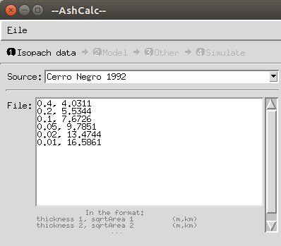
AshCalc requires isopachs to be entered as pairs of values, the thickness of the isopach (measured in metres) and the square root of the area of the isopach (measured in kilometres).
The data can either be entered directly, or alternatively either loaded in from a CSV (comma separated value) file or copy and pasted in by opening the drop down menu Source and clicking Load File...
3.2 Inputting model parameters
The type of model is chosen from the Model drop down menu.
Exponential model
AshCalc finds the best fit for the exponential parameters using segmented least squares regression. It chooses the segment boundaries to ensure the continuity of the resulting curve and, as a result, a poor fit may be observed when the isopach data is not monotonically increasing.
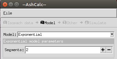
Segments - the number of segments to use in the exponential model. The correct number to use depends on the nature of the isopach data.
Power Law model
AshCalc finds the best fit for the power law parameters using least squares regression.
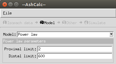
Proximal limit - the proximal limit of integration, see equation. The estimated total volume for a tephra deposit is often very sensitive to the proximal limit of integration in particular and therefore some thought is needed as to the “best” values.
Distal limit - the distal limit of integration, see equation. The distal limit of integration must always be larger the proximal limit of integration.
Weibull model
The equation for T(x) cannot be linearised in the Weibull model, and therefore an optimisation algorithm is needed to find estimates for the values of λ and k. AshCalc uses a random restart stochastic hill-climbing algorithm.
In practice this means that it performs a number of runs. For each run it picks initial random values for λ and k. During the run it repeatedly changes the values for λ and k slightly and seeing if this produces a better solution. If the changes result in a better solution it accepts the changes and continues to try and find another improvement. After a predefined number of iterations the run terminates and the best values found in that run are returned. A number of these runs are performed and the best overall result is returned.
As the algorithm is stochastic AshCalc will return different (but usually similar) results for the Weibull model when run multiple times on the same data. The extent to which the solution fits the data can be judged using the MRSE value (described in the results section).
Correspondingly there is no guarantee that any particular calculation will provide a suitable answer (although with a suitable number of runs and iterations the probability is high). If an unsatisfactory fit is found it is recommended the calculation is performed again, taking into account the suggestions below.
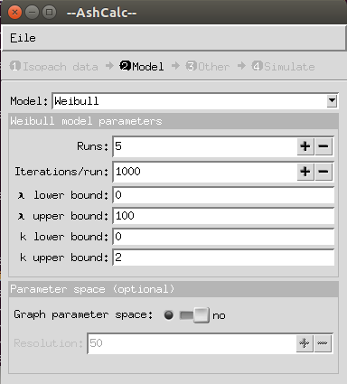
Runs - the number of runs the algorithm performs. Increasing the number of runs increases the probability of a better fit being returned but also increases the computation time required. If poor fits are being returned, it is recommended that the number of runs is increased before the number of iterations per run.
Iterations - the number of iterations per run the algorithm performs. Increasing the number of iterations per run increases the probability of a better fit being returned but also increases the computation time required.
λ lower/upper bounds - the range of values of λ may take while the algorithm searches for the best value.
k lower/upper bounds - the range of values of k may take while the algorithm searches for the best value.
Restricting the bounds for λ and k inappropriately will result in consistently poor fits for the data and inaccurate volume totals.
It is recommended that initially loose bounds are provided (e.g. 0 ≤ λ ≤ 1000, 0 ≤ k ≤ 2). When a reasonable fit for the data is found, the bounds can then be further tightened. For example if it was found that λ = 2.63 and k = 0.849 provided a reasonable fit, the bounds could then be tightened to 1 ≤ λ ≤ 5, 0.5 ≤ k ≤ 1.5.
Investigating the error surface in the results section can often be extremely useful in setting optimal bounds. An in-depth analysis on initial bounds can be found in Costanza Bonadonna’s paper “Plume height, volume, and classification of explosive volcanic eruptions based on the Weibull function” published in the Bulletin of Volcanology (2013).
Graph parameter space: if yes than the AshCalc will create a 2D contour plot/3D graph of the error against parameters λ and k. This allows a visual inspection to help decide on appropriate bounds. It is disabled by default to reduce the computation time required.
Resolution: the resolution at which the resulting contour plot or graph is rendered. At resolution n, an n by n grid of points will be plotted. Increasing the resolution will increase the detail on the plot, but also significantly increase computation time.
4. Results
Each model has several pages of results. The current page may be changed by using the Results drop down menu at the top of the screen.
How well each model fits the data may be estimated using the mean relative squared error (MRSE) of the model, where

A model with MRSE = 0 means that the model perfectly fits the data. The higher the MRSE the less well the model fits. MRSE may be used to compare between models only when they are based on identical isopach data.
4.1 Exponential model
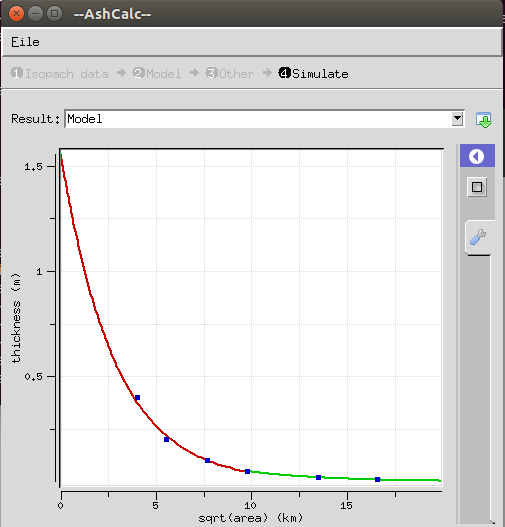
Model
Displays a plot of x, sqrt(Area), vs T(x), thickness. Each segment is displayed in a different colour.
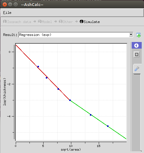
Regression
Displays a plot of sqrt(Area) vs log(T(x)). Each segment is displayed in a different colour. If the data follows a multi-segment exponential distribution then the data points should be closely correlated with the displayed regression lines.
Numerical results
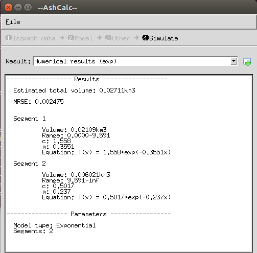
Estimated total volume - the total volume of the deposit in km3 as predicted by the model, obtained by integrating the thickness function with respect to area between 0 and infinity.
MRSE - mean relative squared error, measures how well the model fits the data. A score of zero denotes a perfect fit. Note that accurate comparisons can only be made between models when they use the same isopach data.
Segments - segments are numbered left to right on the model i.e. segment 1 will cover the smallest values of x.
Volume - the volume of the segment in km3.
Range - the range of x-values for which the segment is valid.
c - the value of the segment's coefficient, c.
m - the value of segment's exponent, m.
Equation - the thickness equation for the segment, only valid for x values in the segment's range.
4.2 Power law model
Model
Displays a plot of x, sqrt(Area), vs T(x), thickness. Due to the large values of T(x) for small values of x commonly generated by the power law model and the shortcomings of the Rappture toolkit, it is not always possible to plot the relationship up to the proximal limit of integration. The full curve may be obtained using the equation provided in the numerical results and any common graphing software.
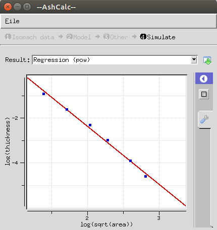
Regression
Displays a plot of log(x) against log(T(x)). If the data follows a power law distribution then the data points should be closely correlated with the line of regression.
Numerical results
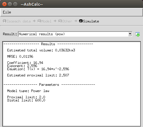
Estimated total volume - the total volume of the deposit in km3 as predicted by the model, obtained by integrating the thickness function with respect to area between 0 and inf.
MRSE - mean relative squared error, measures how well the model fits the data. A score of zero denotes a perfect fit. Accurate comparisons can only be made between models when they use the same isopach data.
c - the value of the coefficient, c.
m - the value of the exponent, m.
Equation - the thickness equation for the model.
Estimated proximal limit - an estimate of the proximal limit derived from the isopach data using the method described in Bonadonna and Houghton (2005).
4.3 Weibull model
Model
Displays a plot of x, sqrt(Area), vs T(x), thickness. Due to the large values of T(x) for small values of x commonly generated by the Weibull model and the shortcomings of the Rappture toolkit, it is not always possible to plot the relationship up to x = 0. The full curve may be obtained using the equation provided in the numerical results and any common graphing software.
Numerical Results
The parameters output for the Weibull model are generated using a non-deterministic algorithm and hence different models may be generated each time. The models obtained can be compared using the MRSE value.
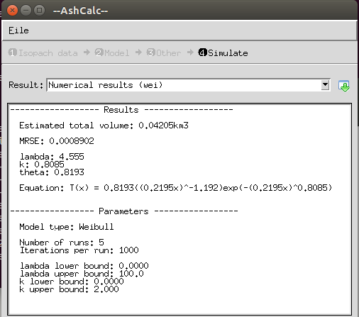
Estimated total volume - the total volume of the deposit in km3 as predicted by the model, obtained by integrating the thickness function with respect to area between 0 and infinity.
MRSE - mean relative squared error, measures how well the model fits the data. A score of zero denotes a perfect fit. Note that accurate comparisons can only be made between models when they use the same isopach data.
lambda - the value of lambda.
k - the value of k.
theta - the value of theta.
Equation - the thickness equation for the model.
Error surface
The error surface is initially displayed as a contour map of the error surface as a function of k and λ. Due to the limitations of Rappture it may be necessary to click the resize button  to the right of the plot to stretch the plot to fill the window.
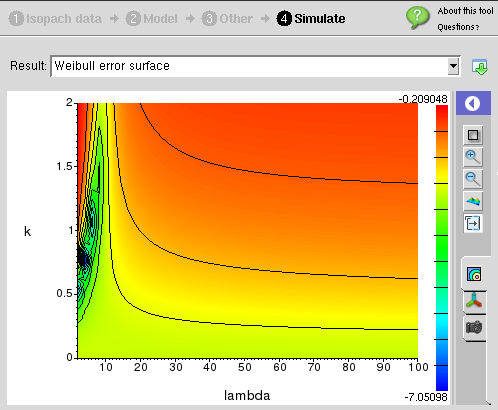
The error surface can be useful in finding appropriate bounds to set for λ and k. For instance in the plot above, it can be seen that the error is minimised in the region for 0 < λ < 20 and 0.5 < k < 1.5.
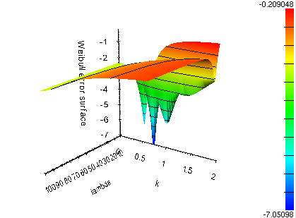
A 3-dimensional version of the error surface may be obtained by clicking the  button to the right of the plot. The example below illustrates the importance of repeatedly refining the values of λ and k, as although there appears to be a clear minimum the three distinct minima are actually artefacts of sampling the function at too low a resolution and in reality the function forms a much smoother valley.
4.4 Downloading the results
The results may be downloaded to your computer using the download button  to the right of the Results drop down menu. Both the graphs and the data may be saved.
5. The offline version of AshCalc
AshCalc was originally implemented purely in Python to be run as an application on the desktop. Both versions use the same Python modules underneath so their results are guaranteed to be consistent.
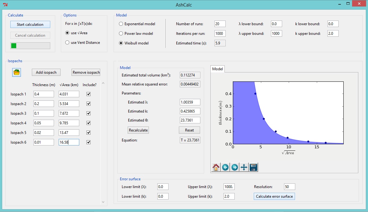
The source code as well as the user manual for the offline version may be found here. The offline version provides extra features not found in this online version.
Advantages
- Dynamic control of the resulting models. After the model is generated the user may adjust the parameters and observe how the model changes.
- Better user interface when manipulating and saving graphs.
- Can be run locally without an internet connection.
Disadvantages
- Requires Python 3 as well as several Python libraries (NumPy, SciPy etc.) installed on the user's computer. Instructions are provided in the download.
Acknowledgements
This work was carried out during the tenure of National Environment Research Council (NERC) research experience placements (to Daggitt and Page). Mather and Pyle acknowledge support from NERC/ESRC grants NE/J020001/1 and NE/J020052/1 (STREVA) and NERC grant NE/I013210/1. Mather further acknowledges funding from the Leverhulme Trust. The authors would like to thank Harriet Rawson and Karen Fontijn for the valuable user feedback during the creation of AshCalc.
Cite this work
Researchers should cite this work as follows:
Daggitt, M. L., Mather, T. A., Pyle, D. M., & Page, S. (2014). AshCalc–a new tool for the comparison of the exponential, power-law and Weibull models of tephra deposition. Journal of Applied Volcanology, 3(1), 7.
Cite this work
Researchers should cite this work as follows: