
Overview: Experimental protocol for Antarctic projections
This page describes the experimental protocol for the ISMIP6 projections that target the upcoming IPCC AR6 assessment. Due to the delay in CMIP6 climate simulations, the initial set of ISMIP6 simulations are based on CMIP5 projections. These CMIP5 models were chosen following the assessment presented in Barthel et al. (2020). As CMIP6 model outputs became available, ISMIP6 included simulations based on these new models. The experimental framework was revised in September 2018 during an ISMIP6 workshop held in Sassenheim (NL).
The revised protocol described in Nowicki et al. (2020) and summarized in Fig. 1 allows for:
- Sampling CMIP scenarios: main focus is on the high emission RCP8.5, but ice sheet evolution in response to low emission RCP2.6 is also investigated.
- Sampling CMIP models: 6 AOGCMs have been selected from the CMIP5 model ensemble: CCSM4, CSIRO-Mk3-6-0, HadGEM2-ES, IPSL-CM5A-MR, MIROC-ESM-CHEM and NorESM1-M. The AOGCMs were identified based on the following steps:
- Present-day climate near Antarctica in agreement with observations (evaluated by model biases over the historical period);
- Sample a diversity of forcing (evaluated by differences in projections and code similarities); and
- Allow only models with RCP8.5 and RCP2.6. The sampling methodology for the CMIP5 models is described in Barthel et al. (2020). As CMIP6 models became available, ISMIP6 prepared dataset for CNRM-CM6 (ssp585 and ssp126), CESM2 (ssp585) and UKEM1-CM6 (ssp585). Unlike for the rigorous analysis for the CMIP5 models, the CMIP6 models were selected because of their availability.
- Sampling ice sheet model uncertainty: “standard” and “open” experiments. The “standard” experiments are based on parameterizations developed by the ocean groups, while “open” experiments utilize the parameterizations already in use by respective ice sheet models. The open experiments are important as they allow to sample the uncertainty in processes that are poorly known, as reflected by different parameterizations.
- Sampling ocean forcing uncertainty: the standard experiments include “high”, “mid” and “low” values for the forcing parameters, as well as two different calibration methods for the basal melt rate parameters (see Jourdain et al., 2020).
- Experiment ranking: This experimental framework results in a series of projections (divided into core and targeted experiments), a historical run and a control run. Not every ice sheet model will be able to carry out the full set of experiments, but they are strongly encouraged to participate in the full suite of core experiments (Table 1, which uses both the “open” and “standard” experiments/parameterizations). Given that the standard experiments requires new implementations, it is OK to only participate with only the open experiments. Similarly, it is OK to only participate with the “standard” experiments. Groups are encouraged to work through the lists presented below (see Table 1 for core experiments, and targeted experiments will follow soon), starting from the top, and complete as many experiments as possible. This approach of combining core and targeted experiments is based on Shannon et al. (2013): it ensures that all groups do a subset of identical experiments, while it also allows faster models to explore the targeted experiment space more fully.
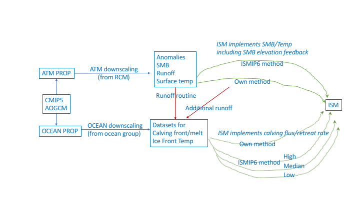
Figure 1: Overview of the Antarctic experimental framework

List of Projections
With the help of the atmosphere and ocean focus groups, a number of CMIP5 AOGCMs have been selected for ISMIP6 standalone ice sheet model projections. Table 1 lists the core experiments which are the minimum contribution expected from ISMIP6 models, in addition to the initialization experiments listed in Table 2.
All groups are encouraged to contribute to the “standard” experiments, but this is not a requirement for participation in ISMIP6. Groups that have their own methods for implementing ocean and atmosphere forcing, are encouraged to do the suite with “open” experiments (1-4), but these are not compulsory. Models that perform the “open” experiments can use the parameterization of their choice to simulate atmospheric and oceanic forcings, but these parameterizations must use the given CMIP5 AOGCM outputs.
Modeling groups that can run many simulations will be encouraged to further explore the ice sheet response using targeted experiments (See Table). These include three additional CMIP5 AOGCMs under RCP8.5, and experiments that explore the ocean forcing uncertainty. Depending on the results of experiments 3 and 7, which consider RCP2.6, additional AOGCMs may be suggested with RCP2.6 for models that are able to do many simulations, but these would be a lower priority than the completing the set of experiments with the 6 AOGCMs for the RCP8.5 scenario. As CMIP6 AOGCMs are becoming available, we are preparing these datasets. The spreadsheet will be updated as new dataset become available. Because there is value in both completing the 6 CMIP5 AOGCMs (to sample the uncertainty in CMIP) and simulations with CMIP6 models, we encourage groups do to as many experiments as possible.
‘Note’: All datasets needed for the core experiments (Table 1) are available on Ghub Globus, as well as the dataset for the additional targeted CMIP5 and CMIP6 models. (See Table)
| Table 1: Core Experiments based on MIROC5, NorESM1-M and HadGEM2-ES | ||||||
| Exp | RCP | AOGCM | Std/open | Ocean Forcing Unc. | Fracture | Note |
| 1 | 8.5 | NorESM1-M | Open | Medium | None | Low atmospheric change and mid-to-high ocean warming |
| 2 | 8.5 | MIROC-ESM-CHEM | Open | Medium | None | High atmospheric changes and median ocean warming |
| 3 | 2.6 | NorESM1-M | Open | Medium | None | Low atmospheric change and mid-to-high ocean warming |
| 4 | 8.5 | CCSM-4 | Open | Medium | None | Large atmospheric warming and variable regional ocean warming |
| 5 | 8.5 | NorESM1-M | Standard | Medium | None | Low atmospheric change an mid-to-high ocean warming |
| 6 | 8.5 | MIROC-ESM-CHEM | Standard | Medium | None | High atmospheric changes and median ocean warming |
| 7 | 2.6 | NorESM1-M | Standard | Medium | None | Low atmospheric change and mid-to-high ocean warming |
| 8 | 8.5 | CCSM4 | Standard | Medium | None | Large atmospheric warming and variable regional ocean warming |
| 9 | 8.5 | NorESM1-M | Standard | High | None | Ocean Forcing Uncertainty, using 95th percentile values |
| 10 | 8.5 | NorESM1-M | Standard | Low | None | Ocean Forcing Uncertainty, using 5ht percentile values |
| 11 | 8.5 | CCSM4 | Open | Medium | Yes | Experiment with ice shelf hydrofracture |
| 12 | 8.5 | CCSM4 | Standard | Medium | Yes | Experiment with ice shelf hydrofracture |
| 13 | 8.5 | NorESM1-M | Standard | PIGL | None | Ocean Forcing Uncertainty, using PIGL, gamma calibration |
Initial state, control run, historical run and projections set up
The core and targeted experiments all start on January 2015 and end in December 2100. The start date follows the CMIP6 protocol for projections, while the end date is constrained by the availability of forcing. In many cases, modelers will need to run a short historical run to bring their models from the “initialization date” to the “projection start date” of January 2015 (see Table 2).
The “initialization date” (or initial state) is left to the modeling groups discretion and can be any time prior to January 2015. The “initialization date” corresponds to the date assigned to the initialization procedure. Groups can reuse their initMIP initialization configuration or generate a new initial state. In the later case, it is important to redo the initMIP schematic experiments 'asmb' and 'abmb' (see initMIP Antarctica and Seroussi et al. 2019), as it will help understanding how a novel initial state contributes to the uncertainty in ice sheet evolution.
A control run (‘ctrl’) is also needed to evaluate model drift. As for initMIP, the control run is obtained by running the model forward, keeping the surface mass balance and ocean forcing used in the initialization technique unchanged. The control run starts from the initial state (typically before 2015) and should last a minimum of 100 years, the same duration as the schematic initMIP experiments. The control run should also be sufficiently long to reach 2100. (See examples in Table 2).
Note that in the event that initMIP schematic experiments and control run are redone as part of the projection setup, then consistency with the projections protocol is more important than consistency with the original initMIP setup. For example, in initMIP bedrock was not allowed to evolve. However, an ISM planning to run the projection with evolving bedrock AND planning to redo the initial state, would also rerun initMIP (ctrl, asmb. abmb) with bedrock change. Similarly, the original initMIP requested 2D output every 5 years, whereas the projections protocol request for yearly values. Therefore if rerunning initMIP, the schematic experiments should be saved yearly.
A single “historical run” is required from each ice sheet model, from which all the projections will branch off. The historical run starts at the initMIP state and ends in December 2014. Groups are free to choose how to run the “historical run” using:
- A reanalysis,
- A historical run from an RCM,
- A historical run from an AOGCM,
- And/or combination of multiple datasets
However, we reject multiple historical runs for each individual AOGCM, because this would very much complicate the forcing strategy and interpretation. As a consequence, in case AOGCM data is used, please decide for one. ISMIP6 provides a climatology for the SMB and surface temperature for each of the AOGCMs used to generate the projection dataset, as well as anomalies.
- For Antarctica, the SMB and temperature climatology corresponds to 1995-2014, to align with the reference period used by AR6. The Antarctic SMB and temperature anomalies are available from 1950. For the Antarctic ocean, the datasets start from 1850 and the climate model climatology corresponds to 1995-2014. Groups that would prefer to use an Antarctica dataset provided by ISMIP6 are recommended to use NorESM-M climatology and anomalies for SMB and surface temperature (in the directory Atmosphere_Forcing/noresm1-m_rcp8.5 directory). See Appendix A2.2 for accessing the forcing data and directories.
- For the ocean, modelers can use observational climatology (Ocean_Forcing/climatology_from_obs_1995-2017 directory), and/or anomalies (Ocean_Forcing/noresm1-m_rcp8.5/1850-1994) directory.
Note that the climate model oceanic climatologies (Ocean_Forcing/noresm1-m_rcp8.5/climatology_1995-2014 directory) are not intended for use by modelers, but are simply provided so that user can see what was subtracted during the datasets preparation, as the ocean forcing data (Ocean_Forcing/noresm1-m_rcp8.5/1850-1994 directory) is the sum of the observational climatology and anomalies.
The “projection control” (ctrl_proj) is an unforced simulation that starts at the same ice sheet state as the projections. It will run until 2100, and is implemented with zero anomalies. It is meant to capture how much drift arises from the historical run.
In most cases the same historical run (and potentially spin-up) can be used for both the standard and open experiments. However, if the implementation of the open and standard experiments requires changes to the ISM that are substantially different (in terms of physics in the ISM), then modelers are allowed to carry out an historical run for the open experiments and an historical run for the standard experiments.
| Table 2: Initialization experiments and examples of different initialization start date | ||||
| Experiment | Note | start 1 (duration) | start 2 (duration) | start 3 (duration) |
| ctrl | Unforced control run, needed for model drift evaluation | 2015 (100 years) | 2005 (100 years) | 1980 (120 years) |
| asmb* | initMIP prescribed surface mass balance anomaly | 2015 (100 years) | 2005 (100 years) | 1980 (100 years) |
| historical | needed to bring model from initial state to projection start date | N/A (0 years) | 2005 (10 years) | 1980 (35 years) |
| ctrl_proj | Unforced control run, starting from January 2015, needed for model drift evaluation following historical | 2015 (85 years) | 2015 (85 years) | 2015 (85 years) |
| *only needed if initial state is different from initMIP | ||||
Atmospheric forcing: SMB and temperature anomalies
ISMIP6 provides surface forcing datasets for the Antarctic ice sheet (AIS) based on CMIP AOGCM simulations. Two approaches are possible: using AOGCM output directly, or re-interpreting the GCM climates through higher-resolution regional climate models (RCMs). The later allows to capture narrow regions at the periphery of the ice sheet with large surface mass balance (SMB) gradients, which are not captured by CMIP5 AOGCMs, and is the technique used for the Greenland ice sheet.
For the Antarctic CMIP5 based projections, RCMs are not used, so SMB anomalies based on AOGCM are directly applied. For CMIP6, many of the AOGCMs that have indicated participation in ISMIP6, now use multiple elevation classes to downscale SMB to finer grid resolution. Once these models have completed the CMIP6 projections, our goal is to include additional ISMIP6 projections using SMB downscaled via elevation class.
For the ISMIP6 projections based on CMIP5 AOGCMs, the surface forcing consists of anomalies in SMB and surface temperature (Fig. 2). SMB is needed by ISMs to compute mass changes at the surface, and surface temperature (i.e., the ice temperature at the base of the snow, as distinct from the 2-m air temperature or skin temperature) is used by many ISMs as an upper boundary condition. The following remarks refer mostly to SMB, but the same comments would generally apply to surface temperature as well.
ISMIP6 provides yearly averaged surface mass balance anomalies, aSMB(x,y,t), along with its components (precipitation, evaporation and runoff), along with SMB climatologies used to compute the anomalies:
aSMB_AOGCM(x,y,t) = SMB_AOGCM(x,y,t) - SMB_CLIM_AOGCM(x,y)
where SMB_AOGCM is the SMB for a given AOGCM and SMB_CLIM_AOGCM is the climatology for that AOGCM. The SMB_CLIM_AOGCM were computed by taking the mean value of all SMB_AOGCM over the reference period (from January 1995 to December 2014). ISMs can use these climatologies for spin-up, if desired, but are free to use their own preferred SMB forcing for spin-up and historical run.
During the run, modelers need to reintroduce the climatology that best fit their simulations. SMB is computed as:
SMB(x,y,t) = SMB_ref(x,y) + aSMB(x,y,t)
where SMB_ref is the SMB that the ice sheet model would have used over the reference period (from January 1995 to December 2014 for Antarctica) and should be the same for all the core and targeted experiments. If a time-dependent SMB is used, then SMB_ref(x,y) is the average over the reference period. If an SMB climatology is used, then SMB_ref(x,y) is simply the climatology. ISMIP6 accept that the use of existing climatologies (or dataset of SMB averaged over many year) may not align with the time period for the AR6 reference period.
However, it is assumed that the differences between climatologies will be less than the inter annual variability from the SMB resulting from the AOGCMs, and thus changes in aSMB. What is important is that the SMB climatology (or SMB_ref) is computed over many years. This assumption also allows for ISM to work with their favorite SMB.
aSMB(x,y,t) is constant over the entire year and changes stepwise at the beginning of every year. SMB climatologies and SMB anomalies are given in units of kg m-2 s-1 (water equivalent), and surface temperature in units of deg K. To convert aSMB to units [m yr-1] typically used in an ice sheet model, multiply the netcdf variable by 31,556,926 s/yr, 1/1000 m3/kg and by the density ratio rho_w/rho_i:
aSMB [m yr^-1^] = aSMB [kg m^-2^ s^-1^] * 31,556,926 / 1000 * (1000/rho_i)
where rho_i is your specific ice density (typically 917.0 or similar).
The datasets can be obtained via Ghub Globus (see instructions in the section above). Files are provided for several resolutions (1 km, 2 km, 4 km, 8 km, 16 km, and 32 km). Modeling groups should use the resolution closest to their native grid to conservatively interpolate data to model (see Appendix 1, below).
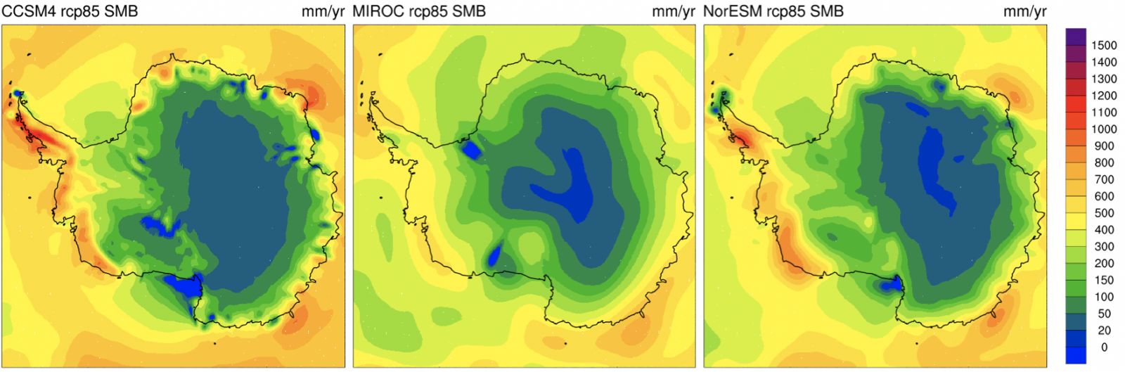
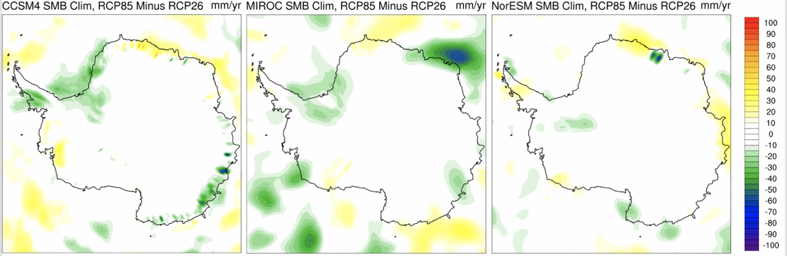
Figure 2: SMB and surface temperature anomalies for CCSM4, MIROC-ESM-CHEM, and NorESM1-M under RCP8.5 and 2.6 (top). SMB climatology for the reference period (January 1995-December 2014) for these models under RCP8.5 (middle), along with difference in SMB climatology between RCP8.5 and 2.6 (bottom).
Oceanic forcing: temperature, salinity, thermal forcing and melt rate parameterization
ISMIP6 provides datasets of extrapolated ocean “ambient” temperature (T), salinity (S) and thermal forcing (TF) from 1850-2100 that are appropriate for present and future ice-shelf cavities. These datasets originate from CMIP models and have been extrapolated under ice shelves, using rules that account for sills and troughs by Xylar Asay-Davis (Fig. 3). The datasets are on the 8 km ISMIP6 Antarctic grid.
Figure 3: Bathymetry and IMBIE2 basins (left) used in the sub-ice shelf extrapolation of ocean temperature (right).
ISMIP6 standard approach
The ISMIP6 standard approach was developed by the Antarctic ocean focus group, and consist of two approaches for the parameterization of basal melt (Jourdain et al., 2020). These ocean melting parameterizations are evaluated for an idealized geometry of the Pine Island glacier in Favier et al. (2019).
The first approach, a non-local quadratic melting parameterization, is the preferred method for ISMIP6 simulations for obtaining melt rates m(x,y) in meters of pure water/yr:
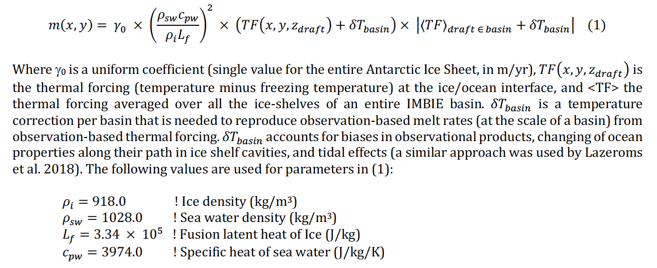
However, an alternative (and easier to implement) takes the form of a local quadratic melting parameterization:
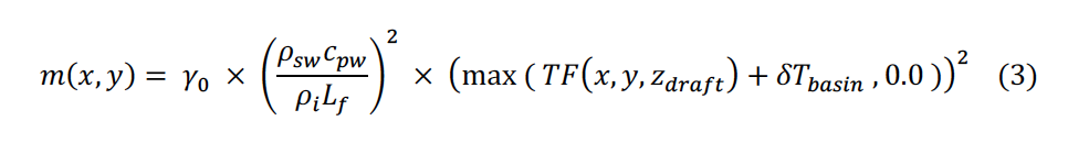
The forcing dataset (for example in the /Ocean_Forcing/noresm1-m_rcp8.5/1995-2100 directory) consist of annual anomalies from the climate models, which were added to the observed climatology (/Ocean_Forcing/climatology_from_obs_1995-2017 directory). Modelers should simply use the data as they are to compute the melt rates using either (1) or (3). In addition to the annual forcing datasets needed for use with these parameterizations, parameters needed to sample the uncertainty in the basal melt are also provided in the /Ocean_Forcing/parameterizations directory.
The files with names *median.nc, *5th_percentiles.nc, *95th_percentiles.nc correspond to the median, low and high cases of the gamma_0 and DeltaT values in the core experiments listed in Table 1.
We test the impact of the calibration method by doing a last experiment in which only a subset of the observation data is used to calibrate the gamma0 coefficient. This choice is motivated by the large impact of melt rate values close to ice shelf grounding lines on the evolution the ice streams feeding them. We choose Pine Island Ice Shelf as it both experiences the largest melt values observed and direct measurements of ocean conditions in the ice shelf cavity are available. We therefore calibrate gamma0 using only the highest 10 basal melt values in Pine Island Ice Shelf, all located close to Pine Island grounding line, in order to assess the sensitivity of the projections to the calibration method. The calibration of the deltaT values is similar to the first calibration method, so that average melt rates for each sector are similar to the melt rates used in the first calibration method and only their spatial distribution varies.
The files with names *_PIGL_gamma_calibration.nc correspond to the experiment 13 listed in Table 1.
Note that the climate model climatologies (Ocean_Forcing/noresm1-m_rcp8.5/climatology_1995-2014 directory) are provided to allow ISMIP6 members to see what was subtracted in the preparation of the ocean forcing dataset, but are not intended to be used in the initialization for example. Instead it is recommended to use the climatology from the observations.
ISMIP6 open approach
The ISMIP6 open approach is used to sample a larger variety of oceanic forcing parameterizations, as it remains an active field of research. Models are free to continue applying the ocean forcing parameterization they used during the model initialization or their preferred method, but should still rely on the ocean forcing datasets provided by ISMIP6 to simulate future ocean conditions. ISMIP6 provides datasets of extrapolated ocean “ambient” temperature (T), salinity (S) and thermal forcing (TF) from 1850-2100 that are appropriate for present and future ice-shelf cavities. These datasets originate from CMIP models and have been extrapolated under ice shelves, using rules that account for sills and troughs by Xylar Asay-Davis (Fig. 3).
The temperature, salinity and thermal forcing data provided for CMIP5 models are the anomalies of each climate model with respect to its January 1995- December 2014 average, added to an observational climatology (based on WOA, EN4 and MEOP datasets). Thus, the data sets are designed to be directly usable by models without the need to compute anomalies or to select reference observations of your own. In such cases, anomalies should be computed with respect to the January 1995- December 2014 average, as this was the period used to anomalize the CMIP5 model input (and slightly different from the time period, 1995-2017, spanned by the observations).
If at all possible, groups using the open approach are encouraged to investigate the uncertainty in their melt parameterization, in a manner similar to the standard approach (where low, median and high values of the gamma_0 and DeltaT parameters are used to investigate the uncertainty in the melt rate. These were obtained by calibration to observed melt.
Antarctic ice shelf fracture
Surface melting can trigger ice shelf collapse (for example, the Larsen B ice shelf in the Antarctic Peninsula). This mechanism is separate from cliff-collapse, but is a precursor to cliff-collapse. Although the mechanisms for Larsen B-style ice shelf collapse are still poorly understood, ISMIP6 provides dataset for ice shelf collapse in the form of a time dependent mask (Figure 4). These datasets were derived from CMIP5 near surface air temperature (tas) following the method described in Trusel et al. (2015), which results in annual surface melt. For ISMIP6, Luke Trussel prepared the bias corrected annual surface melt, which were used to generate the masks. Ice shelves are assumed to collapse following a 10 year period with annual surface melt above 725 mm (Trusel et al., 2015). Some experiments require to model ice shelf collapse and the ISMIP6 masks provided should be used in this case. For the other experiments, ice shelf collapse should not be included.
Models are free to decide on the appropriate method to simulate tributary glaciers’ behavior following the collapse of ice shelves. As the masks were derived from observations, the observed ice shelf may not always corresponds to an ice shelf in the ISM. In the event that the ice shelf collapse mask corresponds to a region which an ISM considers to be grounded (ice sheet), the collapse should not be imposed. Similarly, in the event that applying the mask results in “iceberg” or regions of floating ice shelf that are now detached from the ice shelf, these floating part of the ice should be removed as well.
The datasets can be obtained via Globus under AIS Projections Ice Shelf Fracture datasets
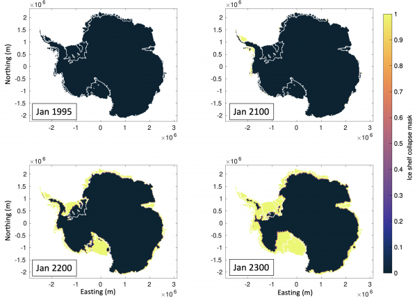
Figure 4: Ice shelf collapse mask for CCSM4 under RCP8.5
Requirements for the projections
Participants can and are encouraged to contribute with different models and/or initialization methods- Models have to be able to prescribe a given SMB anomaly
- Models have to be able to use one of the two ocean parameterizations (non-local or local) proposed for the core experiments.
- The adjustment of SMB due to geometric changes in forward experiments is encouraged.
- Bedrock adjustment in forward experiment is allowed.
- The choice of model input data is unconstrained to allow participants the use of their preferred model setup without modification. Modelers without preferred data set choice can have a look at the ISMIP6 1985432d2dc23d71> page for possible options.
- Participants must submit a README file along with the model outputs as an integral part of the contribution to the ISMIP6. It may be obtained here or requested by email to ismip6@gmail.com. To allow for analysis, any modeling choice needs to be well documented.
Appendix 1 – Output grid definition and interpolation
All 2D data is requested on a regular grid with the following description. Polar stereo-graphic projection with standard parallel at 71° S and a central meridian of 0° W on datum WGS84. The lower left corner is at (-3,040,000 m, -3,040,000 m) and the upper right at (3,040,000 m, 3,040,000 m). This is the same grid used to provide the SMB and basal melting anomaly forcings. The output should be submitted on a resolution adapted to the resolution of the model and can be 32km, 16 km, 8 km, 4 km, 2 km or 1 km. The data will be stored on this resolution for archiving and conservatively interpolated on a 8 km resolution for diagnostic processing by ISMIP6. Output should be provided with single precision.
If interpolation is required in order to transform the SMB forcing (1 km grid data) to your native grid, and transform your model variables to the initMIP output grid (32 km, 16 km, 8 km, 4 km, 2 km, 1 km), it is required that conservative interpolation is used. The motivation for using a common method for all models is to minimize model to model differences due to the choice of interpolation method.
A1.1 Regridding Tools and Tips
An overview of the regridding process can be found on the two Regridding wikis:ISMIP6 is designing tools to help with the regridding. If you need help with conservative interpolation, please email ismip6@gmail.com.
Appendix 2 – Naming conventions, upload and model output data
Please provide:
- one variable per file for all 2D fields and scalar variables
- a completed readme file
- single precision should be used for all output
A2.1 File name convention
File name convention for 2D fields and scalar variables:
<variable>_<IS>_<GROUP>_<MODEL>_<EXP>.nc
File name convention for readme file:
README_<IS>_<GROUP>_<MODEL>.doc
where
<variable> = variable name (e.g. lithk)
<IS> = ice sheet (AIS or GIS)
<GROUP> = group acronym (all upper case or numbers, no special characters)
<MODEL> = model acronym (all upper case or numbers, no special characters)
<EXP> = experiment name (init, ctrl, asmb or abmb)
For example, a file containing the variable “orog” for the Antarctic ice sheet, submitted by group “JPL” with model “ISSM” for experiment “ctrl” would be called:
orog_AIS_JPL_ISSM_ctrl.nc
If JPL repeats the experiments with a different version of the model (for example, by changing the sliding law), it could be named ISSM2, and so forth.
A2.2 Accessing ISMIP6 datasets and submitting model experiments
ISMIP6 datasets are distributed via the Ghub Globus web application. Public datasets can be found in Ghub’s Browse Data page. ISMIP6-specific initMIP Antarctic (and initMIP Greenland and projection data) can be accessed through the Ghub endpoints via Globus UI. To access and download data, one must create a Ghub account and register with Globus. Instructions to create accounts can be referenced in the General ISMIP6 Globus Instructions (v. 2023) instruction document at the end of this wiki.
This documentation provides instructions on how to use Globus to download Ghub data in general, including the ISMIP6 datasets distributed via Ghub. These datasets are from earlier ISMIP6 activities, such as the initMIP, ABUMIP or projections to 2100. ISMIP6 and GHub is partnered with UB CCR to provide access to large datasets. These datasets are described in detail on our Browse Data page. If you have any questions or issues, please contact us by email at ismip6@gmail.com. See more details on Ghub’s Accessing Data wiki. Please also check the suggested text to acknowledge the many scientists and organizations that made the ISMIP6 data possible.
A2.2.1 Where to upload your results
Model results should also be uploaded through Ghub. Once ready to upload your results, you should send an email to ismip6@gmail.com and ask that a new directory be created for your model results. You will then be able to upload your results in this directory using Globus.
A2.2.2 Reducing the size of files
The size of the model files on higher resolution grid can be largely reduced by file compression which will save space on the storage server. An example command is given below and the results before and after. In the examples that follow we can get a factor of 10 compression and for the masks even more given that contiguous masks are highly compressible because they are repeated data. NetCDF files have been designed with compression in mind. A NetCDF file can be compressed and nothing has to be changed in the way that it is read into Matlab or Python (or any other language that uses standard NetCDF read/write libraries).
The nccopy command copies an input netCDF file to an output netCDF file after compressing the file significantly. The ‘-d’ option stands for the deflation level, from 1 (faster but lower compression) to 9 (slower but more compression) and the ‘-s’ option is the shuffling option to improve compression even more. We recommend using ‘d1’ option since this option seems to accomplish the desired compression.
Example of netcdf compression command:
nccopy -d1 -s sftgif_GIS_JPL_ISSMPALEO_historical.nc sftgif_GIS_JPL_ISSMPALEO_historical_c.nc
Example of compression variant, seems to work better for masks:
nccopy -d1 sftgif_GIS_JPL_ISSMPALEO_historical.nc sftgif_GIS_JPL_ISSMPALEO_historical_c.nc
A2.3 Model output variables and README file
The README file is an important contribution to the ISMIP6 submission. It may be obtained here or requested by email to ismip6@gmail.com
A2.3.1 General guidelines
The variables requested in Table A1 serve to evaluate and compare the different models and initialization techniques. Some of the variables may not be applicable for your model, in which case they are to be omitted (with explanation in the README file).
We distinguish between state variables “‘ST”’ (e.g. ice thickness, temperatures and velocities) and flux variables “‘FL”’ (e.g. SMB). State variables should be given as snapshot information at the end of one year for both scalars and 2D variables (for initMIP, 2D variables were only requested over five year periods), while flux variables are to be averaged over the respective periods. Please specify in your README file how your reported flux data has been averaged over time. Ideally, the standard would be go average over all native time steps.
Flux variables are defined positive when the process adds mass to the ice sheet and negative otherwise.
All “missing data” must be assigned the single precision floating point value of 1.e20. Fields should be undefined outside of the ice mask.
If you redo the initMIP experiments (because you have a new initial state for the projections), please save the files at a yearly interval instead of the 5 years interval requested as part of the original initMIP. Also upload your iniMIP results in the projections directory.
A2.3.2 How to record time in historical and projection files
In compliance with CMIP6, time should be defined in “days since “, where must be specified by the user, typically in the form year-month-day (e.g., “days since 1800-1-1”). For simulations meant to represent a particular historical period, set the ‘base time’ to the time at the beginning of the simulation. A historical run initialized with forcing for year 2007 would, for example, have units of “days since 2007-1-1”. For the future scenario runs, retain the same as used in the historical run from which it was initiated.
Note the CF definition for years (section 4.4):
-
common_yearis 365 days -
leap_yearis 366 days -
Julian_yearis 365.25 days -
Gregorian_yearis 365.2425 days -
360_dayhas all years with 360 days divided into 30 day months - Please see the CF link above for other examples on calendar setting in section 4.4.
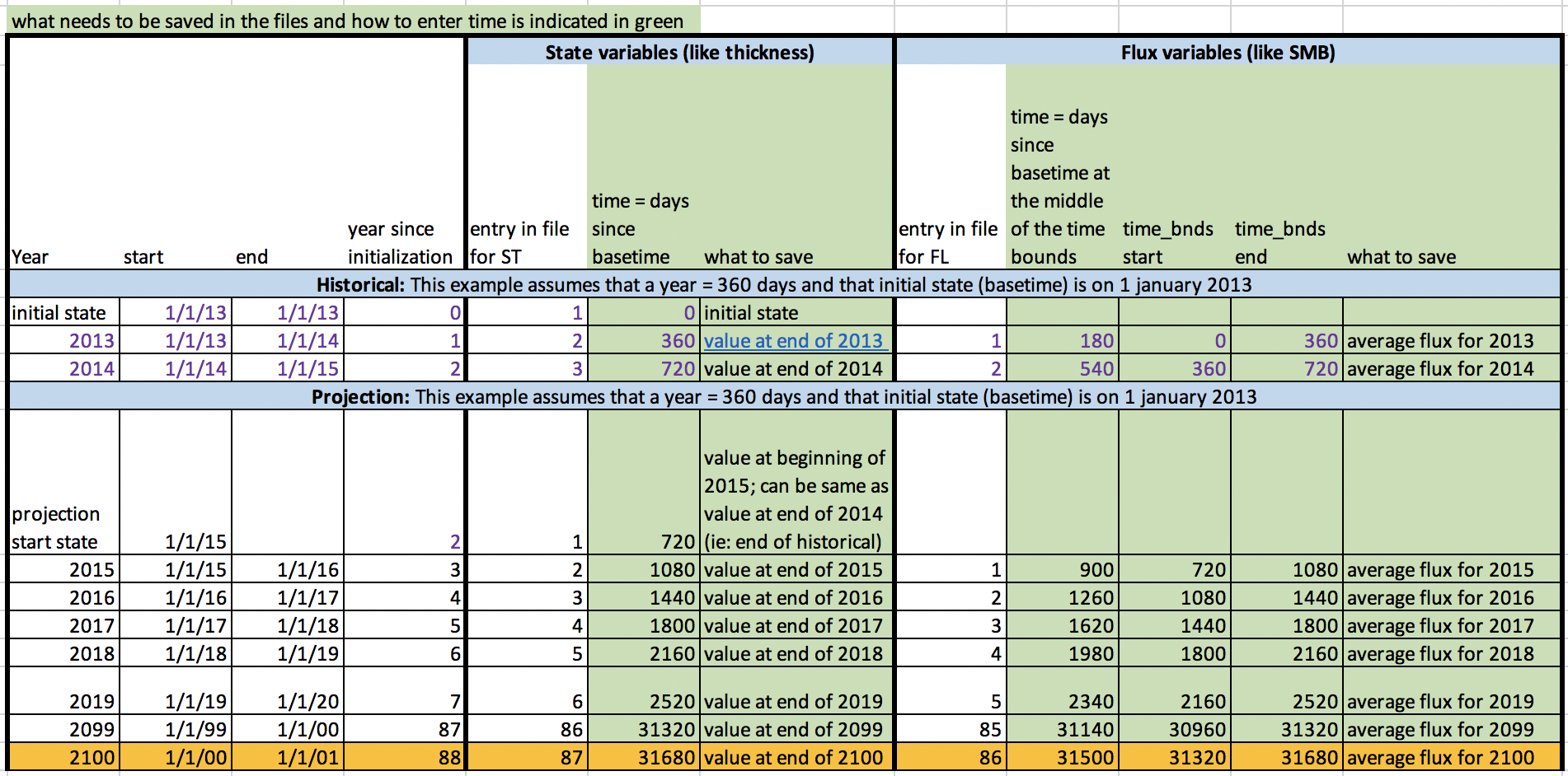
To illustrate a time recording for the historical file and projections for a typical state variable (ST, eg thickness) and flux variable (FL, eg SMB), we assume that our <basetime> is January 1st 2013, and that we use a calendar = 360_days.
Other calendars can be used, but you need to indicate the calendar used in the netcdf, and of course if you use a different calendar, the time entries will be different. What needs to be recorded is shown in green in the Table’ below. For state variables, <time> is the day corresponding to the entry that you are saving since the your <basetime>. For flux variables, since these are averaged over a year, is the day since <basetime> corresponding to the middle of the year, while <time_bnds> records the day since <basetime> at the start and end of a year. Note that in CMIP a full year is typically from first of January to the first of January of the following year.
We also provide below example of what the netcdf would look like for our example..
For state variables, like thickness for the historical:
 dimensions:
    time = UNLIMITED ; // (3 currently)
 variables:
    double time(time) ;
        time:units = "days since 1-1-2013" ; // This date correspond to the example basetime
        time:calendar = "360_day" ; // Other calendars can be used... change here to relevant calendar
        time:axis = "T" ;
        time:long_name = "time" ;
        time:standard_name = "time" ;
 data:
  time = 0, 360, 720; // If you use a different calendar these values will change

=For thickness for the projection=
'''''note''' that the full time entries are not shown, only beginning and end) would be:

 dimensions:
    time = UNLIMITED ;
 variables:
    double time(time) ;
        time:units = "days since 1-1-2013" ; // This date correspond to the example basetime
        time:calendar = "360_day" ; // Other calendars can be used... change here to relevant calendar
        time:axis = "T" ;
        time:long_name = "time" ;
        time:standard_name = "time" ;
 data:
  time = 720, 1080, 1440, …, 31320, 31680; // If you use a different calendar these values will change

=The flux variable, like SMB, would be recorded as the average over a full year, so for the historical:=

 dimensions:
    time = UNLIMITED ; // (2 currently)
    bnds = 2 ;
 variables:
    double time(time) ;
        time:bounds = "time_bnds" ;
        time:units = "days since 1-1-2013 " ; // This date correspond to the example basetime
        time:calendar = "360_day" ; // Other calendars can be used... change here to relevant calendar
        time:axis = "T" ;
        time:long_name = "time" ;
        time:standard_name = "time" ;
    double time_bnds(time, bnds) ;
 data:
  time = 180, 540 ; // If you use a different calendar these values will change.
                              //This is the middle of the time_bnds
  time_bnds =
   0, 360, //If you use a different calendar these values will change.
               //These are the day since basetime at the beginning and end of the year
   360, 720 ;

=For the projection=
'''''note''''' that the full time entries are not shown, only beginning and end):

 dimensions:
    time = UNLIMITED ; //
    bnds = 2 ;
 variables:
    double time(time) ;
        time:bounds = "time_bnds" ;
        time:units = "days since 1-1-2013 " ; // This date correspond to the example basetime
        time:calendar = "360_day" ;  // Other calendars can be used... change here to relevant calendar
        time:axis = "T" ;
        time:long_name = "time" ;
        time:standard_name = "time" ;
    double time_bnds(time, bnds) ;
 variables:
    double time(time) ;
        time:bounds = "time_bnds" ;
 data:
  time = 900, 1260, 1620, ..., 31140, 31500; // If you use a different calendar these values will change.
                                                      //This is the middle of the time_bnds
  time_bnds =
 720, 1080, //If you use a different calendar these values will change.
                  //These are the day since basetime at the beginning and end of the year
 1080, 1440,
 1440, 1800,
 ....
 30960, 31320,
 31320, 31680;
A2.3.3 Table A1: Variable request for ISMIP6
If your quantity does not change with time, then simply save one time entry. An example is geothermal heat flux, which varies in some models but not others.
Model Characteristics The Model Characteristics table can be found here.
| Table A1: Variable request for ISMIP6 projections.
Bold names or “alias” indicate a change compared to initMIP, to align the request with the CMIP6 official MIPtable “IyrAnt” or names in the CF convention. If possible please use the new names, and if not, the name change will occur when your files are checked for CMIP compliance. The first entry should be that from which the simulation starts. Fields such as surface mass balance flux should be what was applied as boundary conditions. |
|||||||
| 2D variables requested yearly as snashots (end of the year) for type ST and as yearly average for type FL. | |||||||
| Variable | Dim | Type | Variable Name | Standard Name | Units | Comment | |
| Ice thickness | x,y,t | ST | lithk | land_ice_thickness | m | The thickness of the ice sheet | |
| Surface elevation | x,y,t | ST | orog | surface_altitude | m | The altitude or surface elevation of the ice sheet | |
| Base elevation | x,y,t | ST | base | base_altitude | m | The altitude of the lower ice surface elevation of the ice sheet | |
| Bedrock elevation | x,y,t | ST | topg | bedrock_altitude | m | The bedrock topography (may change during the projections) | |
| Geothermal heat flux | x,y,t | FL | hfgeoubed | upward_geothermal_heat_flux_in_land_ice alias “upward_geothermal_heat_flux_at_ground_level” | W m-2 | Geothermal Heat flux at the land ice interface (only needed beneath the grounded ice). If this quantity does not change with time, then a single entry is sufficient | |
| Surface mass balance flux | x,y,t | FL | acabf | land_ice_surface_specific_mass_balance_flux | kg m-2 s-1 | Surface Mass Balance flux | |
| Basal mass balance flux beneath grounded ice | x,y,t | FL | libmassbfgr alias “libmassbf” | land_ice_basal_specific_mass_balance_flux | kg m-2 s-1 | Basal mass balance flux (only beneath grounded ice) | |
| Basal mass balance flux beneath floating ice | x,y,t | FL | libmassbffl alias “libmassbf” | land_ice_basal_specific_mass_balance_flux | kg m-2 s-1 | Basal mass balance flux (only beneath floating ice) | |
| Ice thickness imbalance | x,y,t | FL | dlithkdt | tendency_of_land_ice_thickness | m s-1 | dHdt | |
| Surface velocity in x | x,y,t | ST | xvelsurf alias “uvelsurf” | land_ice_surface_x_velocity | m s-1 | u-velocity at land ice surface | |
| Surface velocity in y | x,y,t | ST | yvelsurf alias “vvelsurf” | land_ice_surface_y_velocity | m s-1 | v-velocity at land ice surface | |
| Surface velocity in z | x,y,t | ST | zvelsurf alias “wvelsurf” | land_ice_surface_upward_velocity | m s-1 | w-velocity at land ice surface | |
| Basal velocity in x | x,y,t | ST | xvelbase alias “uvelbase” | land_ice_basal_x_velocity | m s-1 | u-velocity at land ice base | |
| Basal velocity in y | x,y,t | ST | yvelbase alias “vvelbase” | land_ice_basal_y_velocity | m s-1 | v-velocity at land ice base | |
| Basal velocity in z | x,y,t | ST | zvelbase alias “wvelbase” | land_ice_basal_upward_velocity | m s-1 | w-velocity at land ice base | |
| Mean velocity in x | x,y,t | ST | xvelmean alias “uvelmean” | land_ice_vertical_mean_x_velocity | m s-1 | The vertical mean land ice velocity is the average from the bedrock to the surface of the ice | |
| Mean velocity in y | x,y,t | ST | yvelmean alias “vvelmean” | land_ice_vertical_mean_y_velocity | m s-1 | The vertical mean land ice velocity is the average from the bedrock to the surface of the ice | |
| Surface temperature | x,y,t | ST | litemptop alias “litempsnic” | temperature_at_top_of_ice_sheet_model alias “temperature_at_ground_level_in_snow_or_firn” | K | Ice temperature at surface | |
| Basal temperature beneath grounded ice sheet | x,y,t | ST | litempbotgr alias “litempbot” | temperature_at_base_of_ice_sheet_model alias “land_ice_basal_temperature” | K | Ice temperature at base of grounded ice sheet | |
| Basal temperature beneath floating ice shelf | x,y,t | ST | litempbotfl alias “litempbot” | temperature_at_base_of_ice_sheet_model alias “land_ice_basal_temperature” | K | Ice temperature at base of floating ice shelf | |
| Basal drag | x,y,t | ST | strbasemag | land_ice_basal_drag alias “magnitude_of_land_ice_basal_drag” | Pa | Basal drag | |
| Calving flux | x,y,t | FL | licalvf | land_ice_specific_mass_flux_due_to_calving | kg m-2 s-1 | Loss of ice mass resulting from iceberg calving. Only for grid cells in contact with ocean | |
| Ice front melt and calving flux | x,y,t | FL | lifmassbf | land_ice_specific_mass_flux_due_to_calving_and_ice_front_melting | kg m-2 s-1 | Loss of ice mass resulting from ice front melting and calving. Only for grid cells in contact with ocean | |
| Grounding line flux | x,y,t | FL | ligroundf | land_ice_specific_mass_flux_at_grounding_line | kg m-2 s-1 | Loss of grounded ice mass resulting at grounding line. Only for grid cells in contact with grounding line | |
| Land ice area fraction | x,y,t | ST | sftgif | land_ice_area_fraction | 1 | Fraction of grid cell covered by land ice (ice sheet, ice shelf, ice cap, glacier) | |
| Grounded ice sheet area fraction | x,y,t | ST | sftgrf | grounded_ice_sheet_area_fraction | 1 | Fraction of grid cell covered by grounded ice sheet, where grounded indicates that the quantity correspond to the ice sheet that flows over bedrock | |
| Floating ice sheet area fraction | x,y,t | ST | sftflf | floating_ice_shelf_area_fraction alias “floating_ice_sheet_area_fraction” | 1 | Fraction of grid cell covered by ice sheet flowing over seawater | |
| Scalar outputs requested every full year: snapshots for type ST and 1 year averages for type FL. | |||||||
| Total ice mass | t | ST | lim | land_ice_mass | kg | spatial integration, volume times density | |
| Mass above floatation | t | ST | limnsw | land_ice_mass_not_displacing_sea_water | kg | spatial integration, volume times density | |
| Grounded ice area | t | ST | iareagr alias “iareag” | grounded_ice_sheet_area alias “grounded_land_ice_area” | m2 | spatial integration | |
| Floating ice area | t | ST | iareafl alias “iareaf” | floating_ice_shelf_area | m2 | spatial integration | |
| Total SMB flux | t | FL | tendacabf | tendency_of_land_ice_mass_due_to_surface_mass_balance | kg s-1 | spatial integration | |
| Total BMB flux | t | FL | tendlibmassbf | tendency_of_land_ice_mass_due_to_basal_mass_balance | kg s-1 | spatial integration | |
| Total BMB flux beneath floating ice | t | FL | tendlibmassbffl | tendency_of_land_ice_mass_due_to_basal_mass_balance | kg s-1 | spatial integration (computed beneath floating ice only) | |
| Total calving flux | t | FL | tendlicalvf | tendency_of_land_ice_mass_due_to_calving | kg s-1 | spatial integration | |
| Total calving and ice front melting flux | t | FL | tendlifmassbf | tendency_of_land_ice_mass_due_to_calving_and_ice_front_melting | kg s-1 | spatial integration | |
| Total grounding line flux | t | FL | tendligroundf | tendency_of_grounded_ice_mass | kg s-1 | spatial integration | |
Appendix 3 – Participating Models and Characteristics
Antarctica Standalone Ice Sheet Modeling
| Contributors | Model | Group ID | Group |
| Thomas Kleiner, Johannes Sutter, Angelika Humbert | PISM | AWI | Alfred Wegener Institute for Polar and Marine Research, DE /University of Bremen, DE |
| Stephen Price, Matthew Hoffman, Tong Zhang | MALI | DOE | Los Alamos National Laboratory, Los Alamos, USA |
| Ralf Greve, Reinhard Calov | SICOPOLIS | ILTS_PIK | Institute of Low Temperature Science, Hokkaido University, Sapporo, JP, Potsdam Institute for Climate Impact Research, Potsdam, DE |
| Heiko Goelzer, Roderik van de Wal | IMAUICE | IMAU | Utrecht University, Institute for Marine and Atmospheric Research (IMAU), Utrecht, NL |
| Helene Seroussi, Nicole Schlegel | ISSM | JPL | NASA Jet Propulsion Laboratory, Pasadena, USA |
| Aurélien Quiquet, Christophe Dumas | GRISLI | LSCE | Laboratoire des Sciences du Climat et de l’Environnement,Université Paris-Saclay, France |
| William Lipscomb, Gunter Leguy | CISM | NCAR | National Center for Atmospheric Research, Boulder, CO, USA |
| Ronja Reese, Torsten Albrecht, Matthias Mengel, Ricarda Winkelmann | PISM | PIK | Potsdam Institute for Climate Impact Research, DE |
| Helene Seroussi, Mathieu Morlighem, Tyler Pelle | ISSM | UCIJPL | NASA Jet Propulsion Laboratory, Pasadena, USA / University of California Irvine, Irvine, USA |
| Frank Pattyn ,Sainan Sun | FETISH | ULB | Laboratoire de Glaciologie, Université Libre de Bruxelles, Brussels, BE |
| Chen Zhao, Rupert Gladstone, Ben Galton-Fenzi | ELMER | UTAS | University of Tasmania, Australia |
| Jonas Van Breedam, Philippe Huybrechts | AISMPALEO | VUB | Vrije Universiteit Brussel, Brussels, BE |
| Nick Golledge, Dan Lowry | PISM | VUW | Antarctic Research Centre, Victoria University of Wellington, NZ |
References
- Barthel, A., Agosta, C., Little, C.M., Hattermann, T., Jourdain, N.C., Goelzer, H., Nowicki, S., Seroussi, H., Straneo, F. and Bracegirdle, T.J., (2020). CMIP5 model selection for ISMIP6 ice sheet model forcing: Greenland and Antarctica, The Cryosphere, 14(3), 855–879, https://doi.org/10.5194/tc-14-855-2020
- Favier, L.’, Jourdain, N. C., Jenkins, A., Merino, N., Durand, G., Gagliardini, O., Gillet-Chaulet, F., and Mathiot, P.: Assessment of Sub-Shelf Melting Parameterisations Using the Ocean-Ice Sheet Coupled Model NEMO(v3.6)-Elmer/Ice(v8.3), Geosci. Model Dev., https://doi.org/10.5194/gmd-12-2255-2019, 2019.
- Jourdain, N.C., Asay-Davis, X., Hattermann, T., Straneo, F., Seroussi, H., Little, C.M. and Nowicki, S., 2020. A protocol for calculating basal melt rates in the ISMIP6 Antarctic ice sheet projections. The Cryosphere, 14(9), 3111-3134. https://doi.org/10.5194/tc-14-3111-2020
- Nowicki, S., Goelzer, H., Seroussi, H., Payne, A. J., Lipscomb, W. H., Abe-Ouchi, A., Agosta, C., Alexander, P., Asay-Davis, X. S., Barthel, A., Bracegirdle, T. J., Cullather, R., Felikson, D., Fettweis, X., Gregory, J. M., Hattermann, T., Jourdain, N. C., Kuipers Munneke, P., Larour, E., Little, C. M., Morlighem, M., Nias, I., Shepherd, A., Simon, E., Slater, D., Smith, R. S., Straneo, F., Trusel, L. D., van den Broeke, M. R., and van de Wal, R. (2020). Experimental protocol for sea level projections from ISMIP6 stand-alone ice sheet models, The Cryosphere, 14, 2331–2368, https://doi.org/10.5194/tc-14-2331-2020
- Seroussi, H., Nowicki, S., Simon, E., Abe Ouchi, A., Albrecht, T., Brondex, J., Cornford, S., Dumas, C., Gillet-Chaulet, F., Goelzer, H., Golledge, N. R., Gregory, J. M., Greve, R., Hoffman, M. J., Humbert, A., Huybrechts, P., Kleiner, T., Larour, E., Leguy, G., Lipscomb, W. H., Lowry, D., Mengel, M., Morlighem, M., Pattyn, F., Payne, A. J., Pollard, D., Price, S., Quiquet, A., Reerink, T., Reese, R., Rodehacke, C. B., Schlegel, N.-J., Shepherd, A., Sun, S., Sutter, J., Van Breedam, J., van de Wal, R. S. W., Winkelmann, R., and Zhang, T., 2019 initMIP-Antarctica: An ice sheet model initialization experiment of ISMIP6, The Cryosphere., 13, 1441-1471, https://doi.org/10.5194/tc-13-1441-2019
- Shannon, S.R., Payne A.J., Bartholomew I.D., Van Den Broeke M.R., Edwards T.L., Fettweis X., Gagliardini O., Gillet-Chaulet F., Goelzer H., Hoffman M.J., Huybrechts P. (2013) Enhanced basal lubrication and the contribution of the Greenland ice sheet to future sea-level rise, Proceedings of the National Academy of Sciences, 110(35):14156-61.
Acknowledgements
The experimental protocol and datasets for the ISMIP6-Projections-Antarctica standalone ice sheet simulations would not have been possible without the effort of many scientists that have given their time and expertise, and have run models to convert the CMIP5 models output into datasets that standalone ice sheet models can use. ISMIP6 would like to thank the ocean focus group under the leadership of Fiamma Straneo, the atmospheric focus group under the leadership of Bill Lipscomb and Robin Smith, and the CMIP5 model evaluation focus group under the leadership of Alice Barthel. Xylar Asay-Davis, Nicolas Jourdain, Tore Hattermann, Chris Little, Helene Seroussi have been instrumental in the development of the ice shelf basal melt rate parameterization and associated datasets. Erika Simon, Richard Cullather and Sophie Nowicki prepared the atmospheric dataset. Luke Trusel and Helene Seroussi prepared the ice shelf fracture dataset. Alice Barthel, Chris Little, Cecile Agosta, Nicolas Jourdain, and Tore Hattermann provided a rigorous analysis of the CMIP5 models against historical data, which allowed the CMIP5 model evaluation group and the ISMIP6 steering committee to select the CMIP5 models used in this effort.
Finally, we thank the ISMIP6 ice sheet modelers for their feedback on the design of the protocol and their willingness to participate in ISMIP6.
General ISMIP6 Globus Instructions (v. 2023):
Globus_Instructions_ismip6_general_June2023.docx (2 MB, uploaded by Katelyn Eaman 1 year 2 months ago).