
initMIP Overview: Focus on initialization
Earlier large-scale ice sheet experiments e.g. those run during the ice2sea and SeaRISE initiatives have shown that ice sheet initialization can have a large effect on sea-level projections and gives rise to important uncertainties. Improving initialization techniques is currently a field of active research, which makes it difficult to prescribe one technique as the method of choice for ISMIP6. Instead, we first propose a “Come as you are”- approach, which allows participants to contribute with their currently used model setup and initialization technique for intercomparison (initMIP). This, we hope, allows getting modelers involved early in the ISMIP6 process and keeps the workload for participants as low as possible. Furthermore, the proposed schematic experiments may facilitate to document on-going model development. Starting early in the CMIP6 process implies relying on schematic forcing for the initiation experiments that is independent from CMIP6 AOGCM output, which will only become available later on. As accurately modeling Antarctica at continental scale remains challenging, we offer groups interested in participating but unable to run the entire Antarctic ice sheet to focus on specified basins instead. The initMIP-Antarctica is the first in a series of ISMIP6 ice sheet model intercomparison activities and is led by Helene Seroussi.
Goals
- Compare and evaluate the initialization methods used in the ice sheet modeling community
- Estimate uncertainty associated with initialization
- Get the ice sheet modeling community started with ISMIP6 activities
- Document on-going model development, as the simple experiments could be repeated with new model versions
initMIP Antarctica Experimental setup
Experiments are for the large scale or regional Antarctic ice sheet and are designed to allow intercomparison between models of:
(1) the initial state itself and (2) the response in three schematic forward experiments:
-
init: Initialization to present day with method of choice - Schematic forward experiments
-
2a. ctrl: Unforced control run (100 years) -
2b. asmb: Prescribed schematic surface mass balance anomaly (100 years) -
2c. abmb: Prescribed schematic basal melting anomaly under floating ice (100 years)
-
The three forward experiments serve to evaluate the initialization in terms of model drift (2a. ctrl) and response to perturbations (2b. asmb and 2c. abmb). For 2a. ctrl, the models are run forward without any anomaly forcing, such that whatever surface mass balance (SMB) was used in the initialization technique would continue unchanged. The perturbation in 2b. asmb consists of a given surface mass balance anomaly, which has to be applied relative to the initial SMB inherent to the individual initialization technique. The SMB anomaly in 2b. asmb (the same for each model) is schematic and should not be considered as a realistic projection. The perturbation in 2c. abmb consists of a given basal melting anomaly, which has to be applied relative to the initial basal melting inherent to the individual initialization technique and should be applied only to floating ice at any given time of the simulation. The basal melting anomaly for floating ice in 2c. abmb is schematic and should not be considered as a realistic projection. The core experiment duration is set to 100 years.
Regional models
As accurately modeling the entire Antarctic ice sheet remains challenging, we offer groups the option to focus instead on modeling one or more of five regional basins:
- Amundsen Basin
- Amery Basin
- Wilkes Land
- Ronne-Filchner Basin
- Ross Ice Shelf Basin
Experiments and parameters for the regional models are similar to the continental scale models. Interested participants can submit results for any basin. Results should be reported on the same grid as continental scale models to simplify the analysis. Shapefiles with suggested extent of the regional models (starting from the observed ice divide position and consistent with the basins used in the IMBIE2 effort).
Requirements for the experiments
- Participants can and are encouraged to contribute with different models and/or initialization methods.
- Participants can contribute with continental scale models and/or regional models for the regional basins chosen.
- Models have to be able to prescribe a given SMB anomaly.
- Models have to be able to prescribe a given basal melting anomaly under the floating ice only.
- No adjustment of SMB due to geometric changes in forward experiments (i.e. no elevation – SMB feedback is allowed)
- No bedrock adjustment in forward experiment
- The choice of model input data is unconstrained to allow participants the use of their preferred model setup without modification. Modelers without preferred data set choice can have a look at the ISMIP6 page for possible options.
- The specific year of initialization (between 1950 and 2014) is equally unconstrained to allow the use of different observational data sets that may be tied to certain time periods.
Prescribed SMB anomaly
The SMB anomaly can be obtained through the ISMIP6 datasets distributed via the Ghub Globus web application. See the instructions document at the end of this wiki. Modeling groups should use the 1 km version to conservatively interpolate to their model native grid (see Appendix 1, below).
For experiment 2b. asmb, the amplitude of the SMB anomaly is to be implemented as a time dependent function, which increases step-wise every full year (it is therefore independent of the time step in the model):
SMB(t) = SMB_initialization + SMB_anomaly * (floor (t) / 40); for 0 < t < 40 in years
SMB(t) = SMB_initialization + SMB_anomaly * 1.0; for t > 40 years
where SMB_anomaly is the anomaly provided by ISMIP6 and SMB_initialization is the model specific SMB used for the initialization.
The units of SMB_anomaly are (meter ice equivalent/year) with an assumed density of 910 kg/m3 and 31,556,926 s/yr.
Prescribed basal melt anomaly under floating ice
The basal melt anomaly can be obtained via the Ghub Globus endpoints web application on a 1 km grid. Basal melt anomalies are uniform across a basin to accommodate all the possible initial grounding line positions. These anomalies are somewhat similar to the observed basal melt under floating ice, so they lead to a doubling of the ocean induced melting after 40 years for models with initial basal melting close to today’s observations.
For experiment 2c. abmb, the amplitude of the basal melt anomaly is to be implemented as a time dependent function, similar to experiment 2b. abmb The amplitude of the function applied increases step-wise every full year (it is therefore independent of the time step in the model):
basal_melt(t) = basal_melt_model + basal_melt_anomaly * (floor (t) / 40); for 0 < t < 40 in years
basal_melt(t) = basal_melt_model + basal_melt_anomaly * 1.0; for t > 40 years
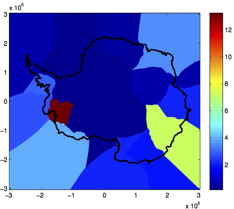
where basal_melt_anomaly is the anomaly provided by ISMIP6 and basal_melt_model is the model specific basal_melt. The anomaly should only be applied on floating ice and should be applied on all floating ice, so that area newly ungrounded should include this anomaly on top of the basal melt applied for the ctrl run (e.g. depth dependent parameterization) as soon as the ice starts floating. The basal melt anomaly is defined over the entire Antarctic grid (see figure below), so newly ungrounded areas or ice front advances should also apply this anomaly as long as the ice is freely floating. The units of basal_melt_anomaly are (meter ice equivalent/year) with an assumed density of 910 kg/m^3 and 31,556,926 s/yr.
Unlike the SMB forcing, the basal melt anomaly is constant per regional basins, so conservative interpolation is not needed and the basal melt anomaly applied should simply equal the value prescribed for each basin. Several version of this anomaly with different grid resolutions (1 km, 2 km, 4 km, 8 km, 16 km and 32 km) are available on the Ghub Globus endpoints web application
Specific uncertainty analysis
At a later stage and informed by the diversity and similarities of participating models, ISMIP6 will suggest further experiments to explicitly address certain aspects of uncertainty in the initialization. It is hoped that participating groups will contribute to these additional experiments, which apply specific perturbations to the initializations. These would take the form of repeating the experiments with systematic perturbations of the initialization choices, for example:
- Boundary conditions and other datasets
- Parameters
- Model structure
- Methods and judgments, e.g. tolerance for data mismatch or drift
Appendix 1 – Output grid definition and interpolation
All 2D data is requested on a regular grid with the following description. Polar stereo-graphic projection with standard parallel at 71° S and a central meridian of 0° W on datum WGS84. The lower left corner is at (-3,040,000 m, -3,040,000 m) and the upper right at (3,040,000 m, 3,040,000 m). This is the same grid used to provide the SMB and basal melting anomaly forcings. The output should be submitted on a resolution adapted to the resolution of the model and can be 32 km, 16 km, 8 km, 4 km, 2 km or 1 km. The data will be stored on this resolution for archiving and conservatively interpolated on a 8 km resolution for diagnostic processing by ISMIP6. Output should be provided with single precision.
If interpolation is required in order to transform the SMB forcing (1 km grid data) to your native grid, and transform your model variables to the initMIP output grid (32 km, 16 km, 8 km, 4 km, 2 km, 1 km), it is required that conservative interpolation is used. The motivation for using a common method for all models is to minimize model to model differences due to the choice of interpolation method.
A1.1 Regridding Tools and Tips
- An overview of the regridding process can be found on the two Regridding pages below.
- Regridding with CDO contains tools and tips that have been used by ISMIP6 members
- Regridding BISICLES output with ESMF and NCO contains other tools and tips
- ISMIP6 is designing tools to help with the regridding.
- If you need help with conservative interpolation, please email ismip6@gmail.com.
Appendix 2 – Naming conventions, upload and model output data
Please provide:
- one variable per file for all 2D fields (no need to provide coordinates)
- all variables in one file for the scalar variables
- a completed readme file
- single precision should be used for all output
A2.1 File name convention
File name convention for 2D fields:
<variable>_<IS>_<GROUP>_<MODEL>_<EXP>.nc
File name convention for scalar variables:
scalar_<IS>_<GROUP>_<MODEL>_<EXP>.nc
File name convention for readme file:
README_<IS>_<GROUP>_<MODEL>.doc
where
<variable> = netcdf variable name (e.g. lithk)
<IS> = ice sheet (AIS or GIS)
<GROUP> = group acronym (all upper case or numbers, no special characters)
<MODEL> = model acronym (all upper case or numbers, no special characters)
<EXP> = experiment name (init, ctrl, asmb, or abmb)
For example, a file containing the scalar variables for the Antarctic ice sheet, submitted by group “JPL” with model “ISSM” for experiment “ctrl” would be called: scalar_AIS_JPL_ISSM_ctrl.nc
If JPL repeats the experiments with a different version of the model (for example, by changing the sliding law), it could be named ISSM2, and so forth.
A2.2 Accessing ISMIP6 datasets and submitting model experiments to Globus
ISMIP6 datasets are distributed via the Ghub Globus web application. Public datasets can be found in Ghub’s Browse Data page. ISMIP6-specific initMIP Antarctic (and initMIP Greenland and projection data) can be accessed through the Ghub endpoints via Globus UI. To access and download data, one must create a Ghub account and register with Globus. Instructions to create accounts can be referenced in the General ISMIP6 Globus Instructions (v. 2023) instruction document at the end of this wiki.
The document provides instructions on how to use Globus to download Ghub data in general, including the ISMIP6 datasets distributed via Ghub. These datasets are from earlier ISMIP6 activities, such as the initMIP, ABUMIP or projections to 2100. ISMIP6 and GHub is partnered with UB CCR to provide access to large datasets. These datasets are described in detail on our Browse Data page. If you have any questions or issues, please contact us by email at ismip6-at-gmail.com. Please also check the suggested text to acknowledge the many scientists and organizations that made the ISMIP6 data possible.
All your model experiments can be uploaded via Globus/Ghub. See more details on Ghub’s Accessing Data wiki. Email ismip6@gmail.com with any questions concerning the above.
A2.3 Model output variables and README file
The README file is an important contribution to the initMIP submission. It may be obtained here or requested by email to ismip6-at-gmail.com
The variables requested in the table below serve to evaluate and compare the different models and initialization techniques. Some of the variables may not be applicable for your model, in which case they are to be omitted (with explanation in the README file).
We distinguish between state variables (ST) (e.g. ice thickness, temperatures and velocities) and flux variables (FL) (e.g. SMB). State variables should be given as snapshot information at the end of one year (for scalars variables) and five year periods (for 2D variables, see table below), while flux variables are to be averaged over the respective periods. Please specify in your README file how your reported flux data has been averaged over time. Ideally, the standard would be go average over all native time steps.
Flux variables are defined positive when the process adds mass to the ice sheet and negative otherwise.
Time should be defined in seconds since the beginning of the run (e.g., units should be “seconds since 2007-01-01 00:00:00”).
| Variable | Dim | Type | Variable Name | Standard Name | Units | Comment |
| 2D variables requested every five years, starting at t=0, snapshots for type ST and as five year average for type FL. | ||||||
| Ice thickness | x,y,t | ST | lithk | land_ice_thickness | m | The thickness of the ice sheet |
| Surface elevation | x,y,t | ST | orog | surface_altitude | m | The altitude or surface elevation of the ice sheet |
| Base elevation | x,y,t | ST | base | base_altitude | m | The altitude of the lower ice surface elevation of the ice sheet |
| Bedrock elevation | x,y,t | ST | topg | bedrock_altitude | m | The bedrock topography (unchanged in forward exps.) |
| Geothermal heat flux | x,y | C | hfgeoubed | upward_geothermal_heat_flux_at_ground_level | W m-2 | Geothermal Heat flux (unchanged in forward exps.) |
| Surface mass balance flux | x,y,t | FL | acabf | land_ice_surface_specific_mass_balance_flux | kg m-2 s-1 | Surface Mass Balance flux |
| Basal mass balance flux | x,y,t | FL | libmassbf | land_ice_basal_specific_mass_balance_flux | kg m-2 s-1 | Basal mass balance flux |
| Ice thickness imbalance | x,y,t | FL | dlithkdt | tendency_of_land_ice_thickness | m s-1 | dHdt |
| Surface velocity in x | x,y,t | ST | uvelsurf | land_ice_surface_x_velocity | m s-1 | u-velocity at land ice surface |
| Surface velocity in y | x,y,t | ST | vvelsurf | land_ice_surface_y_velocity | m s-1 | v-velocity at land ice surface |
| Surface velocity in z | x,y,t | ST | wvelsurf | land_ice_surface_upward_velocity | m s-1 | w-velocity at land ice surface |
| Basal velocity in x | x,y,t | ST | uvelbase | land_ice_basal_x_velocity | m s-1 | u-velocity at land ice base |
| Basal velocity in y | x,y,t | ST | vvelbase | land_ice_basal_y_velocity | m s-1 | v-velocity at land ice base |
| Basal velocity in z | x,y,t | ST | wvelbase | land_ice_basal_upward_velocity | m s-1 | w-velocity at land ice base |
| Mean velocity in x | x,y,t | ST | uvelmean | land_ice_vertical_mean_x_velocity | m s-1 | The vertical mean land ice velocity is the average from the bedrock to the surface of the ice |
| Mean velocity in y | x,y,t | ST | vvelmean | land_ice_vertical_mean_y_velocity | m s-1 | The vertical mean land ice velocity is the average from the bedrock to the surface of the ice |
| Surface temperature | x,y,t | ST | litempsnic | temperature_at_ground_level_in_snow_or_firn | K | Ice temperature at surface |
| Basal temperature | x,y,t | ST | litempbot | land_ice_basal_temperature | K | Ice temperature at base |
| Basal drag | x,y,t | ST | strbasemag | magnitude_of_land_ice_basal_drag | Pa | Magnitude of basal drag |
| Calving flux | x,y,t | FL | licalvf | land_ice_specific_mass_flux_due_to_calving | kg m-2 s-1 | Loss of ice mass resulting from iceberg calving. Only for grid cells in contact with ocean |
| Grounding line flux | x,y,t | FL | ligroundf | land_ice_specific_mass_flux_at_grounding_line | kg m-2 s-1 | Loss of grounded ice mass resulting at grounding line. Only for grid cells in contact with grounding line |
| Land ice area fraction | x,y,t | ST | sftgif | land_ice_area_fraction | 1 | Fraction of grid cell covered by land ice (ice sheet, ice shelf, ice cap, glacier) |
| Grounded ice sheet area fraction | x,y,t | ST | sftgrf | grounded_ice_sheet_area_fraction | 1 | Fraction of grid cell covered by grounded ice sheet, where grounded indicates that the quantity correspond to the ice sheet that flows over bedrock |
| Floating ice sheet area fraction | x,y,t | ST | sftflf | floating_ice_sheet_area_fraction | 1 | Fraction of grid cell covered by ice sheet flowing over seawater |
| Scalar outputs requested every full year, as snapshots for type ST as 1 year averages for type FL. The t=0 value should contain the data of the initialization. | ||||||
| Total ice mass | t | ST | lim | land_ice_mass | kg | spatial integration, volume times density |
| Mass above floatation | t | ST | limnsw | land_ice_mass_not_displacing_sea_water | kg | spatial integration, volume times density |
| Grounded ice area | t | ST | iareag | grounded_ice_sheet_area | m2 | spatial integration |
| Floating ice area | t | ST | iareaf | floating_ice_shelf_area | m2 | spatial integration |
| Total SMB flux | t | FL | tendacabf | tendency_of_land_ice_mass_due_to_surface_mass_balance | kg s-1 | spatial integration |
| Total BMB flux | t | FL | tendlibmassbf | tendency_of_land_ice_mass_due_to_basal_mass_balance | kg s-1 | spatial integration |
| Total calving flux | t | FL | tendlicalvf | tendency_of_land_ice_mass_due_to_calving | kg s-1 | spatial integration |
| Total grounding line flux | t | FL | tendligroundf | tendency_of_grounded_ice_mass | kg s-1 | spatial integration |
Appendix 3 – Participating Models and Characteristics
Antarctica Standalone Ice Sheet Modeling
Model Characteristics
| Model | Numerics | Ice Flow | Initialization | Initial Year | Initial SMB | Basal Sliding | Initial Grid (km) |
| ARC PISM1, PISM2 | FD | HYB | SP | 2000 | RA2 | PL | 16 |
| AWI PISM1Eq, PISM1Pal, PISM2Eq, PISM2Pal | FD | HYB | SP | 2000 | RA2.3 | NP | 16 |
| CPOM BISICLES PRELIM | FV | SSA | DA | 2010 | None | CL | 1-8 |
| ILTS SICOPOLIS | FD | SIA/SSA | SP | 1990 | Arth. | WS | 8 |
| IMAU IMAUICE64 | FD | SSA | SP | 2005 | RA2.3 | VS | 64 |
| JPL1 ISSM | FE | SSA | DA | 2007 | RA2 | WS | 1-50 |
| PSU EQNO MEC | FD | HYB | DA+ SP | 2007 | PDD | WS | 16 |
| PSU GLNO MEC | FD | HYB | SP | 2007 | PDD | WS | 16 |
| UCIJPL ISSM | FE | HO | DA | 2007 | RA2 | WS | 3-50 |
| ULB FETISH | FD | HYB | DA+ SP | 2000 | MAR | WS | 32 |
| VUB AISMPALEO | FD | SIA/SSA | SP | 2000 | PDD | WS | 20 |
| Key | |||||||
| Numerical method: | FD= Finite difference, FE= Finite element, FV= Adaptive mesh refinement | ||||||
| Ice flow: | SIA= Shallow ice approximation, SSA= Shallow shelf approximation, HO= Higher order, HYB= Hybrid SIA-SSA | ||||||
| Initialization: | DA= Data Assimilation, SP= Spin up | ||||||
| Initial SMB: | RA2= RACMO2.1, RA2.3= RACMO2.3, PDD= Positive Degree Day Model, MAR= MAR | ||||||
| Basal sliding: | PL=Pseudo-plastic, NP=Nearly Plastic, VS= Viscous Sliding, WS= Weertman Sliding | ||||||

| Contributors | Model | Group ID | Group |
| Nick Golledge | PISM | ARC | Antarctic Research Centre, Victoria University of Wellington, NZ |
| Thomas Kleiner, Johannes Sutter, Angelika Humbert | PISM | AWI | Alfred Wegener Institute for Polar and Marine Research, DE /University of Bremen, DE |
| Stephen Cornford | BISICLESPRELIM | CPOM | University of Bristol, Centre for Polar Observation and Modelling, UK |
| Christian Rodehacke | PISM0 | DMI | Danish Meteorological Institute, Arctic and Climate, DK |
| Fabien Gillet-Chaulet | ELMER | IGE | Laboratoire de Glaciologie et Géophysique de l’Environnement, FR |
| Ralf Greve | SICOPOLIS | ILTS | Institute of Low Temperature Science, Hokkaido University, Sapporo, JP |
| Heiko Goelzer, Roderik van de Wal, Thomas Reerink | IMAUICE | IMAU | Utrecht University, Institute for Marine and Atmospheric Research (IMAU), Utrecht, NL |
| Nicole Schlegel, Helene Seroussi | ISSM | JPL | NASA Jet Propulsion Laboratory, Pasadena, USA |
| Stephen Price, Matthew Hoffman, Tong Zhang | MALI | LANL | Los Alamos National Laboratory, Los Alamos, USA |
| Aurélien Quiquet, Christophe Dumas | GRISLI | LSCE | Laboratoire des Sciences du Climat et de l’Environnement,Université Paris-Saclay, France |
| William Lipscomb, Gunter Leguy | CISM | NCAR | National Center for Atmospheric Research, Boulder, CO, USA |
| Torsten Albrecht | PISM3PAL | PIK | Potsdam Institute for Climate Impact Research, DE |
| David Pollard | EQNOMEC, GLNOMEC | PSU | Pennsylvania State University EMS Earth and Environmental Systems Institute, Pennsylvania, USA |
| Helene Seroussi, Mathieu Morlighem | ISSM | UCIJPL | NASA Jet Propulsion Laboratory, Pasadena, USA / University of California Irvine, Irvine, USA |
| Sainan Sun, Frank Pattyn | FETISH | ULB | Laboratoire de Glaciologie, Université Libre de Bruxelles, Brussels, BE |
| Jonas Van Breedam, Philippe Huybrechts | AISMPALEO | VUB | Vrije Universiteit Brussel, Brussels, BE |
General ISMIP6 Globus Instructions (v. 2023): Globus_Instructions_ismip6_general_June2023.docx (2 MB, uploaded by Katelyn Eaman 1 year 2 months ago).