initMIP: Focus on initialization
Earlier large-scale ice sheet experiments e.g. those run during ice2sea and SeaRISE initiatives have shown that ice sheet initialization can have a large effect on sea-level projections and gives rise to important uncertainties. Improving initialization techniques is currently a field of active research, which makes it difficult to prescribe one technique as the method of choice for ISMIP6. Our goal is therefore to compare and evaluate the initialization methods used in the ice sheet modeling community and estimate uncertainty associated with initialization.
Instead, we first propose a “Come as you are”- approach, which allows participants to contribute with their currently used model setup and initialization technique for intercomparison (initMIP). We hope this allows getting modelers involved early in the ISMIP6 process and keeps the workload for participants as low as possible. Furthermore, the proposed schematic experiments may facilitate to document on-going model development. Starting early in the CMIP6 process implies relying on schematic forcing for the initiation experiments that is independent from CMIP6 AOGCM output, which will only become available later on.
The initMIP is the first in a series of ISMIP6 ice sheet model intercomparison activities and comprises two separate projects for the:
- Greenland ice sheet: initMIP-Greenland
- Antarctic ice sheet: initMIP-Antarctica
initMIP Goals
- Compare and evaluate the initialization methods used in the ice sheet modeling community
- Estimate uncertainty associated with initialization
- Get the ice sheet modeling community started with ISMIP6 activities
- Document on-going model development, as the simple experiments could be repeated with new model versions
Planning Future ISMIP6 Standalone Experiment: Current thoughts
As described in the main ISMIP6 page, the primary goal of ISMIP6 is to improve projections of sea level rise via projections of the evolution of the Greenland and Antarctic ice sheets under a changing climate, along with a quantification of associated uncertainties (associated with both uncertainty in climate forcing and in the response of the ice sheets).
The standalone ISMIP6 ice sheet experiments are therefore tightly linked with the CMIP6 past and future climate simulation from any AOGCM, and meant to complement the coupled ice sheet-climate simulation.
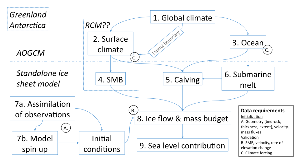
The ISMIP6 flow is shown in the diagram below:
Ways of Providing Atmospheric Forcing
The table below illustrates the many possible ways that Atmospheric Forcings can be provided to an ice sheet model.
Please fill free to indicate other methods!
| Ways of providing SMB forcing for Greenland | |||||
| Method | Advantages | Disadvantages | AOGCM forcing | Actions | |
| 1. | Coupled to a Regional Climate Model. | Full coupling. | (1) Speed of RCM will reduce number of experiments; (2) Limited number of groups could do this. | (1) Lateral boundary conditions for RCM; (2) Sea ice and SSTs. | Find out how groups anticipate doing this. |
| 2. | SMB provided by a Regional Climate Model. | High resolution atmosphere. | (1) Speed of RCM will reduce number of experiments; (2) Needs careful coordination between RCM and ice sheet groups on things such as ice mask; (3) Need to correct for elevation effects; (4) Requires RCM experiments to be completed in advance ideally by several groups. | (1) Lateral boundary conditions for RCM; (2) Sea ice and SSTs. | What RCMs would be available and how many AOGCM-forced experiments would be practical? |
| 3. | SMB calculated by ice-sheet model’s energy-balance scheme. | Fast allowing many experiments. | Not many groups would have this available. | (1) Surface energy fluxes; (2) Precipitation; (3) Hourly/daily. | |
| 4. | SMB calculated by ice-sheet model’s degree-day scheme. | (1) Fast; (2) Easy to implement. | Crude but degree-day factors could be determined from RCMs. | (1) Air temperature and precipitation; (2) Daily/monthly. | Use MAR/RACMO to determine how much DDF varies and if there is a parameterization for this. |
| 5. | Interpolation of SMB directly from AOGCM. | Very fast. | AOGCMs would need to have appropriate physics and output these quantities; resolution issues at margins etc. | SMB terms. | |
| 6. | Adding SMB anomaly from AOGCM to best present day condition. | Very fast. | Present day conditions would come from observation/RCM. This is what SeaRISE did. Still need to decide how to correct for elevation feedback. | SMB terms. | |
Ways of Providing Oceanic Forcing
The table below illustrates the many possible ways that Oceanic Forcings can be provided to an ice sheet model.
Please fill free to indicate new methods!
| Ways of providing SMB forcing for Greenland | |||||
| Method | Advantages | Disadvantages | AOGCM forcing | Actions | |
| 1. | Coupled to a Regional Ocean Model. | Full coupling. | (1) Speed of RCM will reduce number of experiments; (2) Limited number of groups could do this. | Lateral boundary conditions for RCM. | Find out how groups anticipate doing this. |
| 2. | Melt rate + temp provided by a sub ice shelf cavity model. | High resolution ocean. | (1) Speed of RCM will reduce number of experiments; (2) Needs careful coordination between RCM and ice sheet groups on things such as ice mask; (3) Requires RCM experiments to be completed in advance ideally by several groups. | Lateral boundary conditions for RCM. | What RCMs would be available and how many AOGCM-forced experiments would be practical? |
| 3. | Melt rate and heat flux parameterization from box model. | Fast. | Lateral boundary conditions. | ||
| 4. | Use anomalies in surface temp to obtain melt rate (Rignot and Jacob). | (1) Fast; (2) Easy to implement (10 m/a melt per 1 C). | Crude. Cte melt rate for whole ice shelf (but could perhaps combine with Sato and Greve 2012 to get varied sub-melt rate). | Sea surface temperature. | |
| 5. | Apply anomalies from AOGCM to best present day condition (observed or computed melt rates). | Very fast. | What to do when grounding line retreats? etc. | ||


