
Overview
This page describes the experimental protocol for the ISMIP6 2300 projections that focus on simulations of the Antarctic Ice Sheet (AIS) extended to year 2300.
These simulations are based on CMIP5 and CMIP6 climate model outputs, and are a follow-on to the simulations to 2100 described in ISMIP6-Projections-Antarctica and the papers by Nowicki et al. (2020) and Seroussi et al. (2020).
Some experiments use climate forcing from coupled global models that were run until 2300 under CMIP forcing scenarios, while other experiments use repeated forcing from the 2080-2100 period, sampled randomly between 2100 and 2300.
This experiment is now closed and the dataset is available via Ghub/Globus datasets. Please see also the bottom of the page for guidance on usage and how to refer this dataset.
List of Projections
Two CMIP5 models (CCSM4 and HadGEM2) and two CMIP6 models (CESM2 and UKESM) were run with extended high CO2 forcing to 2300 (RCP8.5 and ssp5-85, respectively, for CMIP5 and CMIP6) and were selected for long-term projections. No NorESM1-M extension to 2300 is available, so the extended experiments with NorESM forcing use repeat forcing only.
There are 14 experiments in all. Each experiment ID begins with the prefix ‘AE’ to signify ‘Antarctic extension’. Table 1 lists six Tier-1 experiments that we ask each group to run if possible. This selection includes one run for each of the four climate models with extended forcing to 2300; a low-forcing run for comparison to the high-forcing runs; and one run with repeat forcing from the late 21st century forcing for comparison to runs with extended forcing. If a group is unable to run all six Tier-1 experiments, we ask that they choose a subset.
Table 2 lists an additional eight Tier-2 experiments that we encourage each group to run if resources allow. These include three more experiments with repeat late 21st century forcing, for comparison to the runs with extended forcing. There is one experiment with low emissions (ssp1-26) verextended to 2300, to complement the RCP2.6 experiment in Tier-1. Finally, there are four experiments with prescribed ice-shelf collapse driven by hydrofracture, to compare to the runs without shelf collapse. We excluded shelf-collapse runs from Tier-1 because not all ice sheet models might have this capability.
Modeling groups that can run many simulations are encouraged to further explore the ice sheet response using targeted experiments. For these experiments, groups should repeat the runs in Tables 1 and 2 with either atmospheric or ocean forcing enabled, but not both. This will help us analyze the relative contributions of atmospheric and ocean forcing, especially for the runs with more extreme warming. The experiment numbers are as in Tables 1 and 2, but with a lower-case a or o appended to show which forcing is applied.
For the original ISMIP6 projections, each group was asked to run with a standard sub-shelf melting parameterization based on the method described by Jourdain et al. (2020), and optionally an open parameterization chosen by the group. For the extended Antarctic projections, we no longer prescribe a standard method. Instead, sub-shelf melting schemes are left to the discretion of each group. This change reflects our desire to fully sample the methods in use. As in the original projections, we ask each group to use the thermal forcing data provided by ISMIP6, so that different ice sheet model responses can be attributed to differences in the models rather than the forcing.
Note: All datasets needed for the Tier-2, Tier-2, and targeted experiments are available on Ghub’s Browse Datasets. The same datasets are used for the additional targeted experiments. (See Table)
| Table 1: Tier-1 Experiments | |||||
| Exp | Model | Scenario | Forcing | Collapse | Notes |
| AE01 | NorESM1-M | RCP2.6 | Repeat | No | Low warming scenario |
| AE02 | CCSM4 | RCP8.5 | To 2300 | No | Extended high-emissions CMIP5 scenario |
| AE03 | HadGEM2 | RCP8.5 | To 2300 | No | Extended high-emissions CMIP5 scenario |
| AE04 | CESM2 | ssp5-85 | To 2300 | No | Extended high-emissions CMIP6 scenario |
| AE05 | UKESM | ssp5-85 | To 2300 | No | Extended high-emissions CMIP6 scenario |
| AE06 | UKESM | ssp5-85 | Repeat | No | Repeat forcing for comparison to AE05 |
| Table 2: Tier-2 Experiments | |||||
| Exp | Model | Scenario | Forcing | Collapse | Notes |
| AE07 | NorESM1-M | RCP8.5 | Repeat | No | Extension (with repeat forcing) of ISMIP6-Antarctica Exp 1 |
| AE08 | HadGEM2 | RCP8.5 | Repeat | No | Repeat forcing for comparison to AE03 |
| AE09 | CESM2 | ssp5-85 | Repeat | No | Repeat forcing for comparison to AE04 |
| AE10 | UKESM | ssp1-26 | To 2300 | No | Extended low warming scenario |
| AE11 | CCSM4 | RCP8.5 | To 2300 | Yes | Collapse experiment for comparison to AE02 |
| AE12 | HadGEM | RCP8.5 | To 2300 | Yes | Collapse experiment for comparison to AE03 |
| AE13 | CESM2 | ssp5-85 | To 2300 | Yes | Collapse experiment for comparison to AE04 |
| AE14 | UKESM | ssp5-85 | To 2300 | Yes | Collapse experiment for comparison to AE05 |

Initialization, historical run, control run, and projection runs
All projection experiments start on 1 January 2015 and end on 31 December 2300. The start date follows the CMIP6 protocol for projections, while the end date is constrained by the availability of forcing.
The initialization date (or initial state) is left to each group’s discretion and can be any time before January 2015. The initialization date corresponds to the date assigned to the initialization procedure.
In many cases, a short historical run will be needed to bring the models from the initialization date (say, 1990) to the projection start date of January 2015. Each model configuration should have a single historical run, from which all the projections will branch. Groups are free to choose the forcing for the historical run – for example, using a reanalysis, historical forcing from an RCM or AOGCM, or a combination of multiple datasets. Groups should not carry out a separate historical run for each AOGCM experiment, because this would complicate the forcing strategy and interpretation. Models without a historical run, e.g. that start directly in January 2015, should report their initial conditions as the historical run.
In addition to the projection runs, each model configuration should have a projection control run (ctrl_proj). This is an unforced simulation that starts in January 2015 in the same ice sheet state as the projections, and continues through 2300. It is meant to capture how much drift arises from the historical run. The projection control run is implemented with zero anomalies relative to the 20-year AR6 reference period of January 1995 through December 2014. Below, we offer guidance on choosing SMB and ocean forcing climatologies for the reference period.
Some experiments (#1, 2, 3, 5, 6, 7, 8, 11, 12 and 14 in Tables 1 and 2) use the same forcing for years 2015–2100 as in the original Antarctic projections.
However, the CESM2 ssp5-85 forcing (#4, 9 and 13) has changed, coming from a run with a different atmosphere component (WACCM instead of CAM). The low-emission UKESM forcing (#10) was not part of the original projections. For the experiments with identical 21st century forcing, groups that already ran their models through 2100 can simply continue from 1 January 2101, provided their ice sheet models have not changed. If the models have changed, we ask that groups repeat their initialization and historical run, and then start the projections from 2015.
For groups choosing AOGCM forcing for the initialization or historical run, ISMIP6 provides an SMB and surface temperature climatology, along with anomalies, for each AOGCM used to generate a projection dataset. For Antarctica, the SMB and temperature climatology corresponds to 1995–2014, to align with the AR6 reference period. Antarctic SMB and temperature anomalies are available from 1950. For the Southern Ocean, the datasets start from 1850, and the climate model climatology corresponds to 1995–2014. Groups using an Antarctica dataset provided by ISMIP6 are recommended to use the NorESM1-M climatology and anomalies for SMB and surface temperature (in the directory Atmosphere_Forcing/noresm1-m_rcp8.5). See Appendix A2.2 for accessing the forcing data and directories. For the ocean, modelers can use observational climatology (ISMIP6 2100 dataset forcing directory via /AIS/Ocean_Forcing/climatology_from_obs_1995-2017 directory) and/or anomalies (Ocean_Forcing/noresm1-m_rcp8.5/1850-1994 directory). The climate model ocean climatologies (Ocean_Forcing/noresm1-m_rcp8.5/climatology_1995-2014 directory) are not intended for use by modelers, but are provided so that users can see what was subtracted during the dataset preparation, as the ocean forcing data (Ocean_Forcing/noresm1-m_rcp8.5/1850-1994 directory) is the sum of the observational climatology and model anomalies.
To better sample uncertainties, we encourage groups to submit results using more than one model configuration – for example, from a model run at two or more grid resolutions, or with substantially different physics options. Each configuration would be associated with a separate suite of up to 14 extension experiments. In this case, it is appropriate to do an independent initialization, historical run, and projection control run for each configuration.
Atmospheric forcing: SMB and temperature anomalies
ISMIP6 provides surface forcing datasets for the AIS based on CMIP AOGCM simulations.
Two approaches are possible:
- using AOGCM output directly, or
- re-interpreting the GCM climates through higher-resolution regional climate models (RCMs).
The latter approach, which better captures large surface mass balance (SMB) gradients regions near the periphery of the ice sheet, has been used for ISMIP6 Greenland experiments (Goelzer et al., 2020).
For the Antarctic experiments, RCMs are not used, so SMB anomalies based on AOGCM output are applied directly. Several AOGCMs now use multiple elevation classes to downscale SMB to finer grid resolution over ice sheets. In the future, we may add ISMIP6 experiments using SMB downscaled via elevation class.
For the ISMIP6 projections based on CMIP5 and CMIP6 AOGCMs, the surface forcing consists of anomalies in SMB and surface temperature (illustrated in Fig. 2). SMB is needed by ISMs to compute mass changes at the surface, and surface temperature (i.e., the ice temperature at the base of the snow, as distinct from the 2-m air temperature or skin temperature) is used by many ISMs as an upper boundary condition. The following remarks refer mostly to SMB, but the same comments would generally apply to surface temperature as well.
ISMIP6 provides yearly averaged surface mass balance anomalies, aSMB(x,y,t), along with its components (precipitation, evaporation and runoff), as well as the SMB climatologies used to compute the anomalies:
aSMB_AOGCM(x,y,t) = SMB_AOGCM(x,y,t) - SMB_CLIM_AOGCM(x,y)
where SMB_AOGCM is the SMB for a given AOGCM and SMB_CLIM_AOGCM is the climatology for that AOGCM. The SMB_CLIM_AOGCM were computed by taking the temporal average of all SMB_AOGCM over the reference period (from January 1995 to December 2014). ISMs can use these climatologies for initialization runs, if desired, but are free to use their preferred SMB forcing for these runs.
During the projection run, modelers need to reintroduce the climatology that best fits their simulations. SMB is computed as:
SMB(x,y,t) = SMB_ref(x,y) + aSMB(x,y,t)
where SMB_ref is the SMB that the ice sheet model would have used over the reference period (from January 1995 to December 2014) and should be the same for all experiments. If a time-dependent SMB is used, then SMB_ref(x,y) is the average over the reference period. If an SMB climatology is used, then SMB_ref(x,y) is simply the climatology. ISMIP6 accepts that existing climatologies (or datasets of SMB averaged over many years) may not align exactly with the AR6 reference period.
However, we assume that the differences between climatologies will be less than the inter-annual variability of the SMB derived from the AOGCMs, and thus changes in aSMB. What is important is that SMB_ref is computed over many years. This assumption allows each ISM to use their preferred SMB.
aSMB(x,y,t) is constant over the entire year and changes stepwise at the beginning of the following year. SMB climatologies and anomalies are given in units of kg m-2 s-1 (water equivalent), and surface temperature in units of deg K. To convert aSMB to units [m yr-1 ice] typically used in an ice sheet model, multiply the netcdf variable by 31,556,926 s/yr, 1/1000 m3/kg and by the density ratio ρw/ρi:
aSMB [m yr^-1^] = aSMB [kg m^-2^ s^-1^] * 31,556,926 / 1000 * (1000/ρ^i^)
where ρw = 1000 kg m3 is the density of water, and ρi is your specific ice density (typically 917.0 kg m3 or similar).
The datasets can be obtained from the ISMIP6 2300 Forcing Globus endpoint AIS/Atmosphere_Forcing/. See 2300 Projections Antarctic files at the end of this wiki to set up a Globus account. Files are provided for several resolutions (1 km, 2 km, 4 km, 8 km, 16 km, and 32 km). Modeling groups should use the resolution closest to their native grid to conservatively interpolate the data to the model grid (see Appendix 1, below).
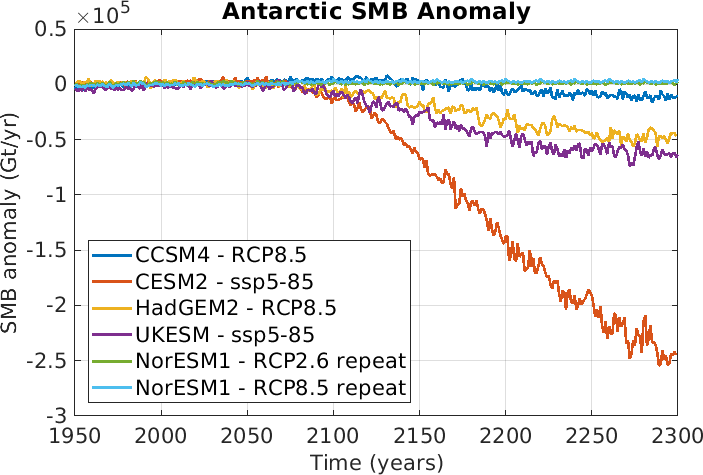
Figure 2a: SMB anomaly (Gt/yr) timeseries, 1950-2300, for CCSM4, CESM2, HadGEM2, UKESM, and NorESM1. All forcings are from high emission scenarios except NorESM1 RCP2.6. NorESM1 anomalies are repeat forcings (see overview).
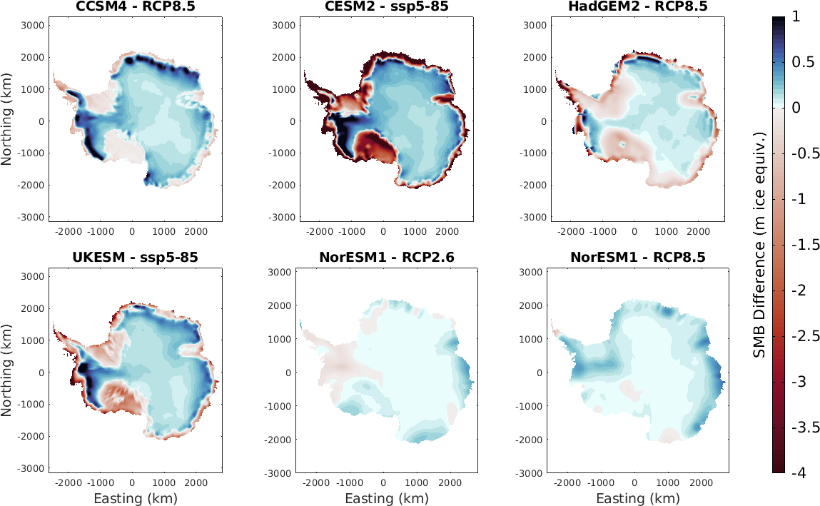
Figure 2b: Change in SMB between the projection start and end date (2300 minus 2015) in units of meters ice equivalent for the AOGCMs shown in Fig. 2a. Note the uneven colorbar.
Oceanic forcing: temperature, salinity, thermal forcing and melt rate parameterization
ISMIP6 provides datasets of extrapolated ocean “ambient” temperature (T), salinity (S) and thermal forcing (TF) from 1850—2300 that are appropriate for present and future ice-shelf cavities. These datasets originate from CMIP models and have been extrapolated under ice shelves by Xylar Asay-Davis, using rules that account for sills and troughs (Fig. 3). The datasets are on the ISMIP6 8-km Antarctic grid. For more information on how the datasets were produced, please see Nowicki et al. (2020), Jourdain et al. (2020), and the ISMIP6 Antarctic Ocean Forcing GitHub.
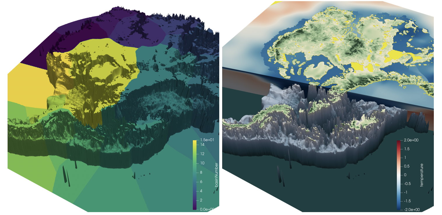
Figure 3: Bathymetry and IMBIE2 basins (left) used in the sub-ice shelf extrapolation of ocean temperature (right).
Modeling groups are free to use their sub-ice-shelf melt rate parameterization of choice, provided that the parameterization uses the ocean forcing datasets (T, S, and TF) provided by ISMIP6. The temperature, salinity and thermal forcing data provided for CMIP5 and CMIP6 models are the anomalies of each model with respect to its January 1995—December 2014 average, added to an observational climatology (based on WOA, EN4 and MEOP datasets). Thus, the datasets can be used directly by models without computing anomalies or selecting reference observations of your own. However, groups might need to compute anomalies. In such cases, anomalies should be computed with respect to the January 1995—December 2014 average, as this period was used to anomalize the CMIP5 model input (and is slightly different from the time period, 1995—2017, spanned by the observations). Groups with multiple submissions using different melt rate parameterizations should carry out all the Tier-1 experiments (Table 1), and optionally the Tier-2 experiments (Table 2), for each submission. Each submission will have an independent initialization and historical run.
Groups may use the quadratic-dependence melt rate parameterization that was developed by the Antarctic ocean focus group and was the standard melt parameterization in ISMIP6 Antarctica (Seroussi et al., 2020). This parameterization is described in detail in Nowicki et al. (2020), Jourdain et al. (2020), ISMIP6-Projections-Antarctica, and Favier et al. (2019). Modeling groups are free to use either median, 5th percentile, or 95th percentile values of the γ,0, and ΔT parameters (provided in /Ocean_Forcing/parameterizations directory), so long as the parameter choice remains consistent. We encourage groups to explore the sensitivity of the melt parameterizations to the values of γ,0, and ΔT. In this case, groups should submit independent initialization and historical runs for each configuration.
The datasets can be obtained from the ISMIP6 2300 Forcing Globus endpoint AIS/Ocean_Forcing/ .
Antarctic ice shelf collapse
Surface melting can trigger ice shelf collapse (for example, the Larsen B ice shelf in the Antarctic Peninsula). This mechanism is distinct from, but a precursor to, cliff collapse. Although the mechanisms for Larsen B-style ice shelf collapse are not well understood, ISMIP6 provides datasets for ice shelf collapse in the form of a time-dependent mask (Fig. 4). These datasets were derived from AOGCM near-surface air temperature (tas) using the method described in Trusel et al. (2015) to compute annual surface melt.
For ISMIP6, Luke Trussel prepared the bias-corrected annual surface melt, which was used to generate the masks. Ice shelves are assumed to collapse following a 10-year period with average surface melt above 725 mm/yr. Some experiments (see Table 2) require modeling ice shelf collapse using the ISMIP6 masks. Ice shelf collapse is included only in Tier-2 experiments and is not a requirement for ISMIP6-2300 participation.
Models are free to decide on the appropriate method to simulate tributary glaciers’ behavior following ice shelf collapse. Since the masks were derived from observations, the observed ice shelf may not always corresponds to an ice shelf in the ISM. In the event that the ice shelf collapse mask corresponds to a region which the ISM considers to be part of the grounded ice sheet, the collapse should not be imposed. Similarly, in the event that applying the mask results in “icebergs” (i.e., regions of floating ice that are now detached from the main ice shelf), these floating regions should be removed.
The datasets can be obtained from the ISMIP6 2300 Forcing Globus endpoint AIS/Ice_Shelf_Fracture/ directory.
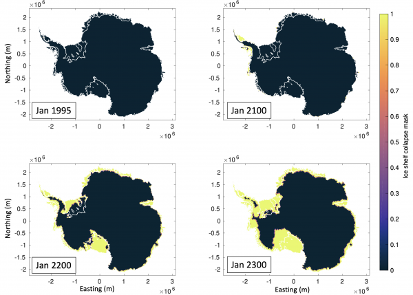
Figure 4: Ice shelf collapse mask for CCSM4 under RCP8.5
Requirements and options for the projections
We encourage participants to contribute results using different models, grid resolutions, physics options, and/or initialization methods.- Models must be able to prescribe a given SMB anomaly.
- Models must be able to use an ocean melt parameterization based on ocean thermal forcing evolving over time, such as the one used for the Tier-1 experiments of the ISMIP6-Antarctica Projections.
- The adjustment of the SMB due to geometric ice-sheet changes in forward experiments is encouraged.
- Bedrock adjustment in forward experiments is allowed.
- The choice of model input data is unconstrained, to allow participants to use their preferred model setup without modification. Modelers without a preferred dataset can look at the ISMIP6 Browse Datasets page for possible options.
- Participants must submit a README file along with the model outputs as an integral part of the contribution to ISMIP6. The README template may be obtained here or requested by email to ismip6@gmail.com. To allow for analysis, models must be well documented.
Appendix 1 – Output grid definition and interpolation
All 2D data is requested on a regular grid with the following description: polar stereographic projection with standard parallel at 71° S and a central meridian of 0° W on datum WGS84. The lower left corner is at (-3,040,000 m, -3,040,000 m) and the upper right at (3,040,000 m, 3,040,000 m). This is the same grid used to provide the 8-km SMB and oceanic forcings. The output should be submitted at a resolution similar to the native model resolution and can be 32 km, 16 km, 8 km, 4 km, 2 km, or 1 km. The data will be stored at this resolution for archiving and conservatively interpolated to the 8-km grid for diagnostic processing by ISMIP6. Output should be provided with single precision.
If interpolation is required to transform the SMB forcing to your native grid, and to transform your model variables to a standard ISMIP6 output grid (32 km, 16 km, 8 km, 4 km, 2 km, or 1 km), conservative interpolation must be used. This requirement minimizes model-to-model differences due to the choice of interpolation method.
A1.1 Regridding Tools and Tips
An overview of the regridding process can be found on the following pages:ISMIP6 is designing tools to help with the regridding. If you need help with conservative interpolation, please email ismip6@gmail.com.
Appendix 2 – Naming conventions, accessing, uploading and modeling output data
Please provide:
- one variable per file for all 2D fields and scalar variables
- a completed readme file
- single precision should be used for all output
A2.1 File name convention
File name convention for 2D fields and scalar variables:
<variable>_<IS>_<GROUP>_<MODEL>_<EXP>.nc
File name convention for readme file:
README_<IS>_<GROUP>_<MODEL>.doc
where
<variable> = variable name (e.g. lithk)
<IS> = ice sheet (AIS or GIS)
<GROUP> = group acronym (all upper case or numbers, no special characters)
<MODEL> = model acronym (all upper case or numbers, no special characters)
<EXP> = experiment name (from the experiment list, e.g. AE01)
For example, a file containing the variable “orog” for the Antarctic ice sheet, submitted by group “JPL” with model “ISSM” for experiment ‘AE05’ would be called:
orog_AIS_JPL_ISSM_AE05.nc
If JPL repeats the experiments with a different version of the model (for example, by changing the sliding law), the model could be named ISSM2, and so forth.
A2.2 Accessing ISMIP6 datasets and accessing the forcing data
ISMIP6 datasets and directories are distributed via the Ghub Globus web application. Public datasets can be found in Ghub’s Browse Data page. ISMIP6-specific initMIP Antarctic (and initMIP Greenland and projection data) can be accessed through the Ghub endpoints via Globus UI. To access and download data, one must create a Ghub account and register with Globus. Instructions to create accounts can be referenced in the 2300 AIS ISMIP6 Globus Instructions (v. Feb 2023) instruction document at the end of this wiki.
This documentation provides instructions on how to use Globus to download Ghub data in general, including the ISMIP6 datasets distributed via Ghub. These datasets are from earlier ISMIP6 activities, such as the initMIP, ABUMIP or projections to 2100. ISMIP6 and GHub is partnered with UB CCR to provide access to large datasets. These datasets are described in detail on our Browse Data page.
If you have any questions or issues, please contact us by email at ismip6@gmail.com. See more details on Ghub’s Accessing Data wiki. Please also check the suggested text to acknowledge the many scientists and organizations that made the ISMIP6 data possible.
A2.2.1 Where to upload your results
Model results should also be uploaded on GHub. Once ready to upload your results, you should send an email to ismip6@gmail.com and ask that a new directory be created for your model results. You will then be able to upload your results in this directory using Globus.
A2.2.2 Reducing the size of files
The size of the model files on higher-resolution grids can be reduced by file compression, which will save space on the storage server. Example commands are given below. Using these commands, we can get 10x compression, and for the masks even more given that contiguous masks contain repeated data. NetCDF files have been designed with compression in mind. A NetCDF file can be compressed without changing the way it is read into Matlab or Python (or any other language that uses standard NetCDF read/write libraries).
The nccopy command copies an input netCDF file to an output netCDF file after compressing the file significantly. The ‘-d’ option stands for the deflation level, from 1 (faster but lower compression) to 9 (slower but more compression). The ‘-s’ option is the shuffling option to improve compression even more. We recommend using the ‘d1’ option, which seems to accomplish the desired compression.
Example of netcdf compression command:
nccopy -d1 -s sftgif_GIS_JPL_ISSMPALEO_historical.nc sftgif_GIS_JPL_ISSMPALEO_historical_c.nc
Example of compression variant, seems to work better for masks:
nccopy -d1 sftgif_GIS_JPL_ISSMPALEO_historical.nc sftgif_GIS_JPL_ISSMPALEO_historical_c.nc
A2.3 Model output variables and README file
The README file is an important contribution to the ISMIP6 submission. A template may be obtained here or requested by email to ismip6@gmail.com.
A2.3.1 General guidelines
The variables requested in Table A1 serve to evaluate and compare the different models and initialization techniques. Some variables may not apply to your model, in which case they can be omitted (with an explanation in the README file).
We distinguish between state variables “ST“ (e.g., ice thickness, temperatures, and velocities) and flux variables “FL” (e.g., SMB). State variables should be given as snapshot information at the end of each year for both scalars and 2D variables (for initMIP, 2D variables were requested only over five-year periods), while flux variables should be averaged over the respective period. Please specify in your README file how your reported flux data has been averaged over time. Ideally, fluxes are averaged over all native model time steps.
Flux variables are defined as positive when the process adds mass to the ice sheet and negative otherwise.
All “missing data” must be assigned the single-precision floating point value of 1e20. Fields should be undefined outside the ice mask.
A2.3.2 How to record time in historical and projection files
In compliance with CMIP6, time should be defined in “days since “, where <basetime> must be specified by the user, typically in the form year-month-day (e.g., “days since 1800-1-1”). For simulations meant to represent a particular historical period, set the ‘base time’ to the time at the beginning of the simulation. A historical run initialized with forcing for year 2007 would, for example, have units of “days since 2007-1-1”. For the future scenario runs, retain the same <basetime> as used in the historical run from which it was initiated.
Note the CF definition for years (section 4.4):
-
common_yearis 365 days, -
leap_yearis 366 days -
Julian_yearis 365.25 days, -
Gregorian_yearis 365.2425 days, -
360_dayyear has 360 days divided into twelve 30-day months - Please see the CF link above for other examples on calendar setting in section 4.4.
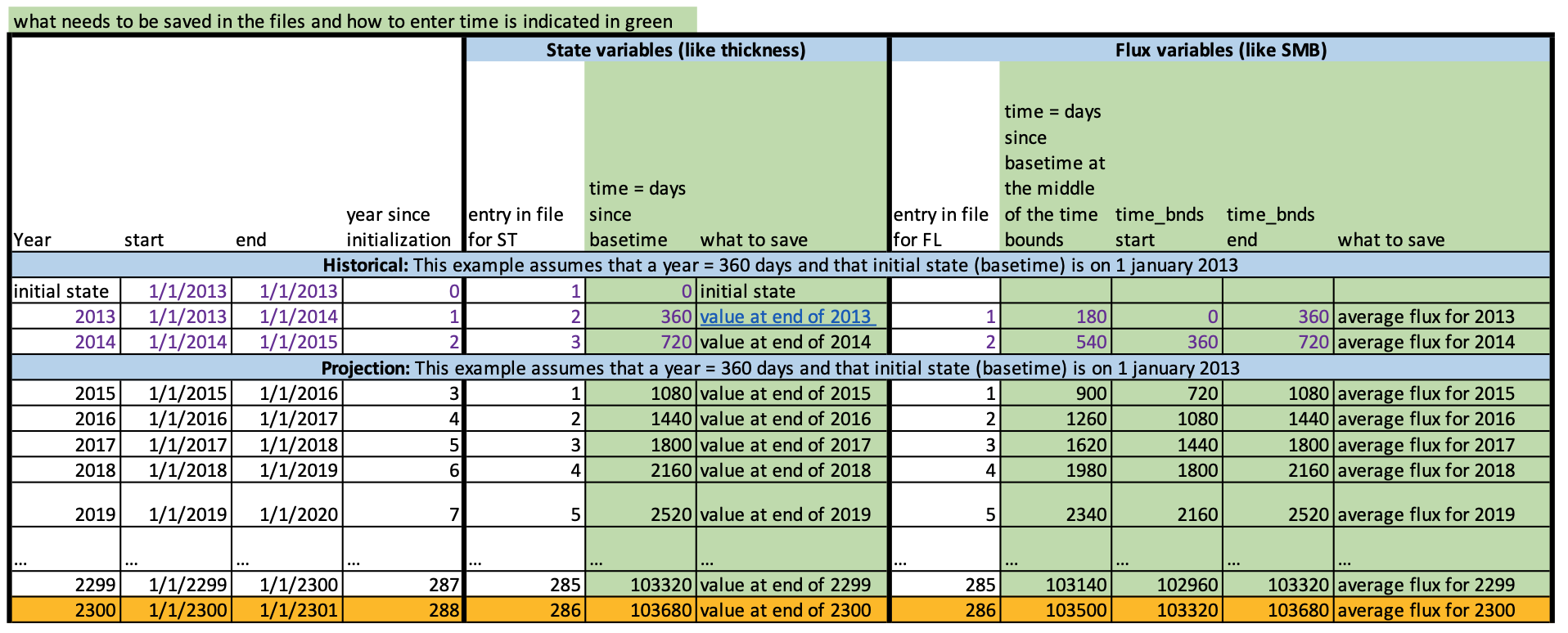
To illustrate a time recording for the historical file and projections for a typical state variable (ST, e.g. thickness) and flux variable (FL, e.g. SMB), we assume that our <basetime> is January 1st 2013, and that we use a calendar = 360_days.
Other calendars can be used, but you need to indicate the calendar used in the netcdf file, and of course if you use a different calendar, the time entries will be different. What needs to be recorded is shown in green in the table below. For state variables, is the day corresponding to the entry that you are saving since the your <basetime>. For flux variables, since these are averaged over a year, is the day since <basetime> corresponding to the middle of the year, while <time_bnds> records the day since at the start and end of a year.
Note:
- In CMIP a full year is typically from first of January to the first of January of the following year. We also provide below an example of what the
netcdfwould look like for our example. - The end of the historical run should not be included at the beginning of the projections to avoid repetitions of the same values. This allows to merge together the different periods without having repeated entries. Models that do not have a historical period and start directly in January 2015 should still submit a historical run with one time step containing the model’s initial conditions.
For state variables, like thickness for the historical:
dimensions:
    time = UNLIMITED ; // (3 currently)
 variables:
    double time(time) ;
        time:units = "days since 1-1-2013" ; // This date correspond to the example basetime
        time:calendar = "360_day" ; // Other calendars can be used... change here to relevant calendar
        time:axis = "T" ;
        time:long_name = "time" ;
        time:standard_name = "time" ;
 data:
  time = 0, 360, 720; // If you use a different calendar these values will change
For thickness for the projection
note: that the full time entries are not shown, only beginning and end) would be:
dimensions:
    time = UNLIMITED ;
 variables:
    double time(time) ;
        time:units = "days since 1-1-2013" ; // This date correspond to the example basetime
        time:calendar = "360_day" ; // Other calendars can be used... change here to relevant calendar
        time:axis = "T" ;
        time:long_name = "time" ;
        time:standard_name = "time" ;
 data:
  time = 720, 1080, 1440, …, 103320, 103680; // If you use a different calendar these values will change
The flux variable, like SMB, would be recorded as the average over a full year, so for the historical:
 dimensions:
    time = UNLIMITED ; // (2 currently)
    bnds = 2 ;
 variables:
    double time(time) ;
        time:bounds = "time_bnds" ;
        time:units = "days since 1-1-2013 " ; // This date correspond to the example basetime
        time:calendar = "360_day" ; // Other calendars can be used... change here to relevant calendar
        time:axis = "T" ;
        time:long_name = "time" ;
        time:standard_name = "time" ;
    double time_bnds(time, bnds) ;
 data:
  time = 180, 540 ; // If you use a different calendar these values will change.
                              //This is the middle of the time_bnds
  time_bnds =
   0, 360, //If you use a different calendar these values will change.
               //These are the day since basetime at the beginning and end of the year
   360, 720 ;
For the projection
note: that the full time entries are not shown, only beginning and end):
 dimensions:
    time = UNLIMITED ; //
    bnds = 2 ;
 variables:
    double time(time) ;
        time:bounds = "time_bnds" ;
        time:units = "days since 1-1-2013 " ; // This date correspond to the example basetime
        time:calendar = "360_day" ;  // Other calendars can be used... change here to relevant calendar
        time:axis = "T" ;
        time:long_name = "time" ;
        time:standard_name = "time" ;
    double time_bnds(time, bnds) ;
 variables:
    double time(time) ;
        time:bounds = "time_bnds" ;
 data:
  time = 900, 1260, 1620, ..., 103140, 103500; // If you use a different calendar these values will change.
                                                      //This is the middle of the time_bnds
  time_bnds =
 720, 1080, //If you use a different calendar these values will change.
                  //These are the day since basetime at the beginning and end of the year
 1080, 1440,
 1440, 1800,
 ....
 102960, 103320,
 103320, 103680;
A2.3.3 Table A1: Variable request for ISMIP6
If your quantity does not change with time, then simply save one time entry. An example is geothermal heat flux, which varies in some models but not others.
Model Characteristics The Model Characteristics table can be found here.
| Table A1: Variable request for ISMIP6 projections.
Bold names or “alias” indicate a change compared to initMIP, to align the request with the CMIP6 official MIPtable “IyrAnt” or names in the CF convention. If possible please use the new names, and if not, the name change will occur when your files are checked for CMIP compliance. The first entry should be that from which the simulation starts. Fields such as surface mass balance flux should be what was applied as boundary conditions. |
|||||||
| Variable | Dim | Type | Variable Name | Standard Name | Units | Comment | |
| 2D variables requested yearly as snapshots (end of the year) for type ST and as yearly average for type FL. | |||||||
| Ice thickness | x,y,t | ST | lithk | land_ice_thickness | m | The thickness of the ice sheet | |
| Surface elevation | x,y,t | ST | orog | surface_altitude | m | The altitude or surface elevation of the ice sheet | |
| Base elevation | x,y,t | ST | base | base_altitude | m | The altitude of the lower ice surface elevation of the ice sheet | |
| Bedrock elevation | x,y,t | ST | topg | bedrock_altitude | m | The bedrock topography (may change during the projections) | |
| Geothermal heat flux | x,y,t | FL | hfgeoubed | upward_geothermal_heat_flux_in_land_ice alias “upward_geothermal_heat_flux_at_ground_level” | W m-2 | Geothermal Heat flux at the land ice interface (only needed beneath the grounded ice). If this quantity does not change with time, then a single entry is sufficient | |
| Surface mass balance flux | x,y,t | FL | acabf | land_ice_surface_specific_mass_balance_flux | kg m-2 s-1 | Surface Mass Balance flux | |
| Basal mass balance flux beneath grounded ice | x,y,t | FL | libmassbfgr’ alias “libmassbf” | land_ice_basal_specific_mass_balance_flux | kg m -2 s-1 | Basal mass balance flux (only beneath grounded ice) | |
| Basal mass balance flux beneath floating ice | x,y,t | FL | libmassbffl alias “libmassbf” | land_ice_basal_specific_mass_balance_flux | kg m-2 s-1 | Basal mass balance flux (only beneath floating ice) | |
| Ice thickness imbalance | x,y,t | FL | dlithkdt | tendency_of_land_ice_thickness | m s-1 | dHdt | |
| Surface velocity in x | x,y,t | ST | xvelsurf alias “uvelsurf” | land_ice_surface_x_velocity | m s-1 | u-velocity at land ice surface | |
| Surface velocity in y | x,y,t | ST | yvelsurf alias “vvelsurf” | land_ice_surface_y_velocity | m s-1 | v-velocity at land ice surface | |
| Surface velocity in z | x,y,t | ST | zvelsurf alias “wvelsurf” | land_ice_surface_upward_velocity | m s-1 | w-velocity at land ice surface | |
| Basal velocity in x | x,y,t | ST | xvelbase alias “uvelbase” | land_ice_basal_x_velocity | m s-1 | u-velocity at land ice base | |
| Basal velocity in y | x,y,t | ST | yvelbase alias “vvelbase” | land_ice_basal_y_velocity | m s-1 | v-velocity at land ice base | |
| Basal velocity in z | x,y,t | ST | zvelbase alias “wvelbase” | land_ice_basal_upward_velocity | m s-1 | w-velocity at land ice base | |
| Mean velocity in x | x,y,t | ST | xvelmean alias “uvelmean” | land_ice_vertical_mean_x_velocity | m s-1 | The vertical mean land ice velocity is the average from the bedrock to the surface of the ice | |
| Mean velocity in y | x,y,t | ST | yvelmean alias “vvelmean” | land_ice_vertical_mean_y_velocity | m s-1 | The vertical mean land ice velocity is the average from the bedrock to the surface of the ice | |
| Surface temperature | x,y,t | ST | litemptop alias “litempsnic” | temperature_at_top_of_ice_sheet_model alias “temperature_at_ground_level_in_snow_or_firn” | K | Ice temperature at surface | |
| Basal temperature beneath grounded ice sheet | x,y,t | ST | litempbotgr alias “litempbot” | temperature_at_base_of_ice_sheet_model alias “land_ice_basal_temperature” | K | Ice temperature at base of grounded ice sheet | |
| Basal temperature beneath floating ice shelf | x,y,t | ST | litempbotfl alias “litempbot” | temperature_at_base_of_ice_sheet_modelalias “land_ice_basal_temperature” | K | Ice temperature at base of floating ice shelf | |
| Basal drag | x,y,t | ST | strbasemag | land_ice_basal_drag alias “magnitude_of_land_ice_basal_drag” | Pa | Basal drag | |
| Calving flux | x,y,t | FL | licalvf | land_ice_specific_mass_flux_due_to_calving | kg m-2 s-1 | Loss of ice mass resulting from iceberg calving. Only for grid cells in contact with ocean | |
| Ice front melt and calving flux | x,y,t | FL | lifmassbf | land_ice_specific_mass_flux_due_to_calving_and_ice_front_melting | kg m-2 s-1 | Loss of ice mass resulting from ice front melting and calving. Only for grid cells in contact with ocean | |
| Grounding line flux | x,y,t | FL | ligroundf | land_ice_specific_mass_flux_at_grounding_line | kg m-2 s-1 | Loss of grounded ice mass resulting at grounding line. Only for grid cells in contact with grounding line | |
| Land ice area fraction | x,y,t | ST | sftgif | land_ice_area_fraction | 1 | Fraction of grid cell covered by land ice (ice sheet, ice shelf, ice cap, glacier) | |
| Grounded ice sheet area fraction | x,y,t | ST | sftgrf | grounded_ice_sheet_area_fraction | 1 | Fraction of grid cell covered by grounded ice sheet, where grounded indicates that the quantity correspond to the ice sheet that flows over bedrock | |
| Floating ice sheet area fraction | x,y,t | ST | sftflf | floating_ice_shelf_area_fraction alias “floating_ice_sheet_area_fraction” | 1 | Fraction of grid cell covered by ice sheet flowing over seawater | |
| Scalar outputs requested every full year: snapshots for type ST and 1 year averages for type FL. | |||||||
| Total ice mass | t | ST | lim | land_ice_mass | kg | spatial integration, volume times density | |
| Mass above floatation | t | ST | limnsw | land_ice_mass_not_displacing_sea_water | kg | spatial integration, volume times density | |
| Grounded ice area | t | ST | iareagr alias “iareag” | grounded_ice_sheet_area alias “grounded_land_ice_area” | m2 | spatial integration | |
| Floating ice area | t | ST | iareafl alias “iareaf” | floating_ice_shelf_area | m2 | spatial integration | |
| Total SMB flux | t | FL | tendacabf | tendency_of_land_ice_mass_due_to_surface_mass_balance | kg s-1 | spatial integration | |
| Total BMB flux | t | FL | tendlibmassbf | tendency_of_land_ice_mass_due_to_basal_mass_balance | kg s-1 | spatial integration | |
| Total BMB flux beneath floating ice | t | FL | tendlibmassbffl | tendency_of_land_ice_mass_due_to_basal_mass_balance | kg s-1 | spatial integration (computed beneath floating ice only) | |
| Total calving flux | t | FL | tendlicalvf | tendency_of_land_ice_mass_due_to_calving | kg s-1 | spatial integration | |
| Total calving and ice front melting flux | t | FL | tendlifmassbf | tendency_of_land_ice_mass_due_to_calving_and_ice_front_melting | kg s-1 | spatial integration | |
| Total grounding line flux | t | FL | tendligroundf | tendency_of_grounded_ice_mass | kg s-1 | spatial integration | |
Appendix 3 – Participating Models and Characteristics
Antarctica Standalone Ice Sheet Modeling for 2300 Projections
The list of participating models will be added as simulations are submitted.
References
- Barthel, A., Agosta, C., Little, C.M., Hattermann, T., Jourdain, N.C., Goelzer, H., Nowicki, S., Seroussi, H., Straneo, F. and Bracegirdle, T.J. (2020): CMIP5 model selection for ISMIP6 ice sheet model forcing: Greenland and Antarctica, The Cryosphere, 14(3), 855–879, https://doi.org/10.5194/tc-14-855-2020.
- Favier, L., Jourdain, N. C., Jenkins, A., Merino, N., Durand, G., Gagliardini, O., Gillet-Chaulet, F., and Mathiot, P. (2019): Assessment of Sub-Shelf Melting Parameterisations Using the Ocean-Ice Sheet Coupled Model NEMO(v3.6)-Elmer/Ice(v8.3), Geosci. Model Dev., https://doi.org/10.5194/gmd-12-2255-2019.
- Jourdain, N.C., Asay-Davis, X., Hattermann, T., Straneo, F., Seroussi, H., Little, C.M. and Nowicki, S. (2020): A protocol for calculating basal melt rates in the ISMIP6 Antarctic ice sheet projections. The Cryosphere, 14(9), 3111-3134. https://doi.org/10.5194/tc-14-3111-2020.
- Nowicki, S., Goelzer, H., Seroussi, H., Payne, A. J., Lipscomb, W. H., Abe-Ouchi, A., Agosta, C., Alexander, P., Asay-Davis, X. S., Barthel, A., Bracegirdle, T. J., Cullather, R., Felikson, D., Fettweis, X., Gregory, J. M., Hattermann, T., Jourdain, N. C., Kuipers Munneke, P., Larour, E., Little, C. M., Morlighem, M., Nias, I., Shepherd, A., Simon, E., Slater, D., Smith, R. S., Straneo, F., Trusel, L. D., van den Broeke, M. R., and van de Wal, R. (2020): Experimental protocol for sea level projections from ISMIP6 stand-alone ice sheet models, The Cryosphere, 14, 2331–2368, https://doi.org/10.5194/tc-14-2331-2020.
- Seroussi, H., Nowicki, S., Simon, E., Abe Ouchi, A., Albrecht, T., Brondex, J., Cornford, S., Dumas, C., Gillet-Chaulet, F., Goelzer, H., Golledge, N. R., Gregory, J. M., Greve, R., Hoffman, M. J., Humbert, A., Huybrechts, P., Kleiner, T., Larour, E., Leguy, G., Lipscomb, W. H., Lowry, D., Mengel, M., Morlighem, M., Pattyn, F., Payne, A. J., Pollard, D., Price, S., Quiquet, A., Reerink, T., Reese, R., Rodehacke, C. B., Schlegel, N.-J., Shepherd, A., Sun, S., Sutter, J., Van Breedam, J., van de Wal, R. S. W., Winkelmann, R., and Zhang, T. (2019): initMIP-Antarctica: An ice sheet model initialization experiment of ISMIP6, The Cryosphere., 13, 1441-1471, https://doi.org/10.5194/tc-13-1441-2019.
- Seroussi, H., Nowicki, S., Payne, A. J., Goelzer, H., Lipscomb, W. H., Abe-Ouchi, A., Agosta, C., Albrecht, T., Asay-Davis, X., Barthel, A., Calov, R., Cullather, R., Dumas, C., Galton-Fenzi, B. K., Gladstone, R., Golledge, N. R., Gregory, J. M., Greve, R., Hattermann, T., Hoffman, M. J., Humbert, A., Huybrechts, P., Jourdain, N. C., Kleiner, T., Larour, E., Leguy, G. R., Lowry, D. P., Little, C. M., Morlighem, M., Pattyn, F., Pelle, T., Price, S. F., Quiquet, A., Reese, R., Schlegel, N.-J., Shepherd, A., Simon, E., Smith, R. S., Straneo, F., Sun, S., Trusel, L. D., Van Breedam, J., van de Wal, R. S. W., Winkelmann, R., Zhao, C., Zhang, T., and Zwinger, T. (2020): ISMIP6 Antarctica: a multi-model ensemble of the Antarctic ice sheet evolution over the 21st century, The Cryosphere, 14, 3033–3070, https://doi.org/10.5194/tc-14-3033-2020.
Acknowledgements
The experimental protocol and datasets for the ISMIP6-Projections2300-Antarctica standalone ice sheet simulations would not have been possible without the effort of many scientists who have given their time and expertise, and have run models to convert the CMIP5 and CMIP6 model outputs into datasets that standalone ice sheet models can use.
ISMIP6 would like to thank the ocean focus group under the leadership of Fiamma Straneo, the atmospheric focus group under the leadership of William Lipscomb and Robin Smith, and the CMIP5 model evaluation focus group under the leadership of Alice Barthel. Xylar Asay-Davis, Nicolas Jourdain, Tore Hattermann, Chris Little, and Helene Seroussi were instrumental in the development of the ice shelf basal melt rate parameterization and associated datasets. Erika Simon, Richard Cullather and Sophie Nowicki prepared the atmospheric dataset. Luke Trusel and Helene Seroussi prepared the ice shelf fracture dataset. Alice Barthel, Chris Little, Cecile Agosta, Nicolas Jourdain, and Tore Hattermann provided a rigorous analysis of the CMIP5 models against historical data, which allowed the CMIP5 model evaluation group and the ISMIP6 steering committee to select the CMIP5 models used in this effort.
Finally, we thank the ISMIP6 ice sheet modelers for their feedback on the design of the protocol and their willingness to participate in ISMIP6.
How to obtain the 2300 AIS ISMIP6 dataset
The dataset for this suite of experiments is currently distributed via Ghub/Globus in a manner similar to the other ISMIP6 datasets. If you use the dataset, please reference the ISMIP6 protocol paper (Nowicki et al. 2020), the model selection (Barthel et al., 2020) and the Antarctic basal melt (Jourdain et al. 2020) and the community publication (Seroussi et al., 2024). The work from CMIP6 should also be recognized and we suggest text to include in any acknowledgement section in our publication page. Please also consider asking for an ISMIP6 contribution number, so that we can include your work on our publication page.