
Overview: Experimental protocol for Greenland projections
This page describes the experimental protocol for the ISMIP6 projections that target the upcoming IPCC AR6 assessment. Due to the delay in CMIP6 climate simulations, the initial set of ISMIP6 simulations are based on CMIP5 projections. These CMIP5 models were chosen following the assessment presented in Barthel et al. (2020). As CMIP6 model outputs became available, ISMIP6 included simulations based on these new models. The experimental framework was revised in September 2018 during an ISMIP6 workshop held in Sassenheim (NL).
The revised protocol – described in Nowicki et al. (2020) and summarized in Figure 1 allows for:
- Sampling CMIP scenarios: main focus is on the high emission RCP8.5, but ice sheet evolution in response to low emission RCP2.6 is also investigated.
- Sampling CMIP models: 6 AOGCMs have been selected from the CMIP5 model ensemble. The AOGCMs were identified based on the following steps:
- Present plausible climates near Greenland (evaluated by model biases over the historical period);
- Have the data at the temporal resolution needed for RCM downscaling;
- Sample a diversity of forcing (evaluated by differences in projections and code similarities); and
- Allow only models with RCP8.5 and ideally with RCP2.6. The sampling methodology for the CMIP5 models is described in Barthel et al. (2020). As CMIP6 models became available, ISMIP6 prepared dataset for CNRM-CM6 (ssp585 and ssp126), CESM2 (ssp585) and UKEM1-CM6 (ssp585). Unlike for the rigorous analysis for the CMIP5 models, the CMIP6 models were selected because of their availability.
- Sampling ice sheet model uncertainty: “standard” and “open” experiments. The “standard” experiments are based on parameterizations developed by the ocean focus group, while “open” experiments utilize the parameterizations already in use by respective ice sheet models. The open experiments are an important contribution as the use of different parameterizations reflect the uncertainty in our current understanding of ice-ocean interactions.
- Sampling ocean forcing uncertainty: the standard experiments include “high”, “mid” and “low” parameters (see Slater et al. 2019 and Slater et al. 2020).
- Experiment ranking: This experimental framework results in a series of projections (divided into core and targeted experiments), a historical run and a control run. Not every ice sheet model will be able to carry out the full set of experiments, but they are strongly encouraged to participate in the full suite of core experiments (Table 1, which uses both the “open” and “standard” experiments/parameterizations). Given that the standard experiments requires new implementations, it is OK to only participate with only the open experiments. Similarly, it is OK to only participate with the “standard” experiments. Groups are encouraged to work through the lists presented below (see Table 1 for core experiments, and targeted experiments will follow soon), starting from the top, and complete as many experiments as possible. This approach of combining core and targeted experiments is based on Shannon et al. (2013): it ensures that all groups do a subset of identical experiments, while it also allows faster models to explore the targeted experiment space more fully.
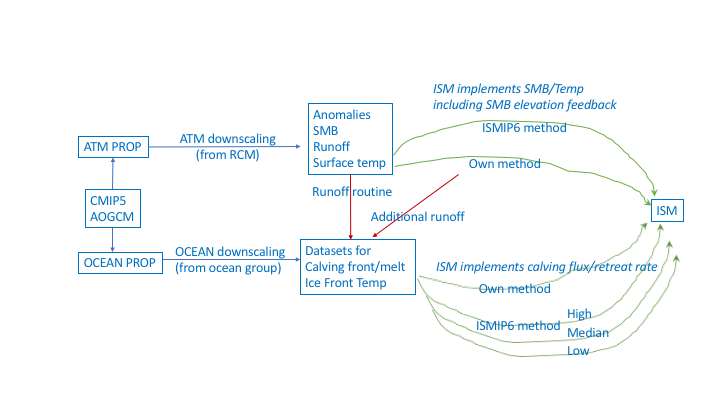
Figure 1: Overview of the Greenland experimental framework
List of Projections
With the help of the atmosphere and ocean focus groups, a number of CMIP5 AOGCMs have been selected for ISMIP6 standalone ice sheet model projections. Table 1 lists the core experiments which are the minimum contribution expected from ISMIP6 models, in addition to the initialization experiments listed in Table 2.
All groups are encouraged to contribute to the “standard” experiments. Groups that have their own methods for implementing ocean and atmosphere forcing, are encouraged to do the suite with “open” experiments (1-4), but these are not compulsory. Models that perform the “open” experiments can use the parameterization of their choice to simulate atmospheric and oceanic forcings, but these parameterizations must use the given CMIP5 AOGCM outputs.
Modeling groups that can run many simulations will be encouraged to further explore the ice sheet response using targeted experiments (See Table and Nowicki et al. (2020)). These include three additional CMIP5 AOGCMs under RCP8.5, and experiments that explore the ocean forcing uncertainty. As CMIP6 AOGCMs became available, a selected number of CMIP6 AOGCMs were also prepared. Because there is value in both completing the 6 CMIP5 AOGCMs (to sample the uncertainty in CMIP) and simulations with CMIP6 models, we encourage groups do to as many experiments as possible.
| Table 1: Core Experiments based on MIROC5, NorESM1-M and HadGEM2-ES | |||||
| Exp | RCP | AOGCM | Std/open | Ocean Forcing Unc. | Note |
| 1 | 8.5 | MIROC5 | Open | Medium | Expected largest response to SMB, median ocean warming |
| 2 | 8.5 | NorESM | Open | Medium | Low atmosphere change, low ocean warming |
| 3 | 2.6 | MIROC5 | Open | Medium | Expected largest response to SMB, median ocean warming |
| 4 | 8.5 | HadGEM2-ES | Open | Medium | Expected median response to SMB, median ocean warming |
| 5 | 8.5 | MIROC5 | Standard | Medium | Expected largest response to SMB, median ocean warming |
| 6 | 8.5 | NorESM | Standard | Medium | Low atmosphere changes, low ocean warming |
| 7 | 2.6 | MIROC5 | Standard | Medium | Expected largest response to SMB, median ocean warming |
| 8 | 8.5 | HadGEM2-ES | Standard | Medium | Expected median response to SMB, median ocean warming |
| 9 | 8.5 | MIROC5 | Standard | High | Ocean Forcing Uncertainty |
| 10 | 8.5 | MIROC5 | Standard | Low | Ocean Forcing Uncertainty |
Initial state, control run, historical run and projections set up
The core and targeted experiments all start on January 2015 and end in December 2100. The start date follows the CMIP6 protocol for projections, while the end date is constrained by the availability of forcing. In many cases, modelers will need to run a short historical run to bring their models from the “initialization date” to the “projection start date” of January 2015.
The “initialization date” (or initial state) is left to the modeling groups discretion and can be any time prior to January 2015. The “initialization date” corresponds to the date assigned to the initialization procedure. Groups can reuse their initMIP initialization configuration or generate a new initial state. In the later case, it is important to redo the initMIP schematic experiments
'asmb' (see initMIP Greenland and Goelzer et al. 2018), as it will help understanding how a novel initial state contributes to the uncertainty in ice sheet evolution.
Note that ISMIP6 has a new standard grid (horizontal resolution of 1 km on projection EPSG:3413), which is different than that used in initMIP-Greenland. The revised datasets for the initMIP ‘asmb’ forcing for the new grid can be obtained from Ghub Globus endpoints. We have changed to the new grid because its projection is standardized and used by many observational datasets that are key input for ice sheet models.
A control run (‘ctrl’) is also needed to evaluate model drift. As for initMIP, the control run is obtained by running the model forward, keeping the surface mass balance and ocean forcing used in the initialization technique unchanged. The control run starts from the initial state (typically before 2015) and should last a minimum of 100 years, the same duration as the schematic initMIP experiments. The control run should also be sufficiently long to reach 2100. (See examples in Table 2).
Note that in the event that initMIP schematic experiments and control run are redone as part of the projection setup, then consistency with the projections protocol is more important than consistency with the original initMIP setup. For example, in initMIP bedrock was not allowed to evolve. However, an ISM planning to run the projection with evolving bedrock AND planning to redo the initial state, would also rerun initMIP (ctrl, asmb) with bedrock change. Similarly, the original initMIP requested 2D output every 5 years, whereas the projections protocol request for yearly values. Therefore if rerunning initMIP, the schematic experiments should be saved yearly.
A single “historical run” is required for each ice sheet model, from which all the projections will branch off. The historical run starts at the initMIP state and ends in December 2014. Groups are free to choose how to run the “historical run”, using a reanalysis, a historical run from an RCM, a historical run from an AOGCM or combination of multiple datasets.
However, we reject multiple historical runs for each individual AOGCM, because this would very much complicate the forcing strategy and interpretation. As a consequence, in case AOGCM data is used, please decide for one. ISMIP6 provides a climatology for the SMB and surface temperature for each of the AOGCMs used to generate the projection dataset, as well as anomalies. Groups that would like to use an ISMIP6 Greenland dataset for initialization and historical run are recommended to use MIROC5.
Note that the SMB and temperature climatology corresponds to January 1960-December 1989 because the ice sheet is assumed in steady state with the climate during this period. To give a concrete example of a historical run that seems to work well: The ice sheet is initialized to a steady state in 1960. RCM anomalies (here RACMO) are applied from 1960 – 2014 on top of the SMB assumed during initialization (here RACMO average 1960-1990). Other SMB products forced with reanalysis data (e.g. MAR) are expected to work equally well.
The “projection control“ (ctrl_proj) is an unforced simulation that starts at the same ice sheet state as the projections. It will run until 2100, and is implemented with zero anomalies. It is meant to capture how much drift arises from the historical run.
In most cases the same historical run (and potentially spin-up) can be used for both the standard and open experiments. However, if the implementation of the open and standard experiments requires changes to the ISM that are substantially different (in terms of physics in the ISM), then modelers are allowed to carry out an historical run for the open experiments and an historical run for the standard experiments.
| Table 2: Initialization experiments and examples of different initialization start date | ||||
| Experiment | Note | start 1 (duration) | start 2 (duration) | start 3 (duration) |
| ctrl | Unforced control run, needed for model drift evaluation | 2015 (100 years) | 2005 (100 years) | 1980 (120 years) |
| asmb* | initMIP prescribed surface mass balance anomaly | 2015 (100 years) | 2005 (100 years) | 1980 (100 years) |
| historical | needed to bring model from initial state to projection start date | N/A (0 years) | 2005 (10 years) | 1980 (35 years) |
| ctrl_proj | Unforced control run, starting from January 2015, needed for model drift evaluation following historical | 2015 (85 years) | 2015 (85 years) | 2015 (85 years) |
| *only needed if initial state is different from initMIP | ||||
Atmospheric forcing: SMB and temperature anomalies
Introduction
ISMIP6 provides anomalies of SMB and temperature, along with associated climatology, as it allows for an experimental framework that is applicable to a diverse set of ice sheet models.
Before applying SMB anomalies, ISMs need to be initialized by applying a baseline SMB (either a time series or a climatology). ISMIP6 provides SMB climatologies for the reference period (January 1960 to December 1989) from the same models computing the anomalies. This reference period for Greenland SMB was chosen because the ice sheet is assumed to be in steady state with the surrounding climate over that period. ISMs can use these climatologies for spin-up, if desired, but are free to use their own preferred SMB forcing.
Elevation feedbacks have been shown to be important in century-scale simulations. For example, Le clec’h et al. (2019) considered differences between no coupling (SMB independent of z), one-way coupling (i.e., correcting SMB outputs for ISM topography changes), and two-way coupling (allowing ice-sheet topographic changes to feed back on the RCM simulation.) Their results suggest that one-way coupling is sufficient to represent elevation feedbacks until the end of the 21st century. For large topographic changes on longer timescales, it might be necessary to incorporate two-way feedbacks, which are beyond the scope of the standalone ISM effort (but will be considered in the ISMIP6 coupled GCM-ISM experiments).
Provided forcing data sets
ISMIP6 provides surface forcing datasets for the Greenland ice sheet (GrIS) based on CMIP AOGCM simulations. The AOGCM output is re-interpreted through higher-resolution regional climate models (RCMs). The later allows to capture narrow regions at the periphery of the Greenland ice sheet with large surface mass balance (SMB) gradients, which are not captured by CMIP5 AOGCMs. For CMIP6, many of the AOGCMs that have indicated participation in ISMIP6 now use multiple elevation classes to downscale SMB to finer grid resolution. Once these models have completed the CMIP6 projections, our goal is to include additional ISMIP6 projections using SMB downscaled via elevation class.
For the ISMIP6 projections based on CMIP5 AOGCMs, the surface forcing datasets were prepared by Xavier Fettweis, using the MAR regional climate model. RCM downscaling can take account of modest future topography/extent changes, and thus cope with the fact that individual ISM runs may not use exactly the same geometry. All RCM runs use a fixed topography, but vertical SMB gradients for each grid cell are derived using the method described by Franco et al. (2012). At each location the vertical gradient in SMB is found by summing and averaging pairwise differences in the nearest neighbor cells. This vertical gradient is used to downscale the SMB (15 km) to a finer grid (1 km), allowing resolution of steep topography that is not represented accurately on the coarse grid. The same information is used to parameterize the SMB-height feedback in the projections. In addition, MAR calculates a potential SMB term for areas that are outside of the observed ice sheet extent, allowing application to ISMs with ice lying outside the MAR ice-sheet mask. However, experience with initMIP has shown that large variations in ice-sheet extent can lead to considerable bias in the projections. We therefore propose a method (see below) for models with large difference from the observed ice sheet extent, to remap the SMB anomaly to the individual modeled ice sheet geometry.
The atmospheric forcings consist of annual anomalies of SMB (aSMB) and surface temperature, along with a fields to represent the dependence of SMB and surface temperature on elevation (dSMBdz, dTdz). SMB is needed by ISMs to compute mass changes at the surface, and surface temperature (i.e., the ice temperature at the base of the snow, as distinct from the 2-m air temperature or skin temperature) is used by many ISMs as an upper boundary condition in the ice temperature calculations. ISMIP6 also provides the climatologies that were used to calculate the anomalies:
aSMB_AOGCM(x,y,t) = SMB_AOGCM(x,y,t) - SMB_CLIM_AOGCM(x,y),
where SMB_AOGCM is the downscaled SMB for a given AOGCM (using MAR RCM) and SMB_CLIM_AOGCM is the corresponding climatology. The SMB_CLIM_AOGCM were computed by taking the mean value of all SMB_AOGCM over the reference period (from January 1960 to December 1989). ISMs can use these climatologies for spin-up, if desired, but are free to use their own preferred SMB forcing for spin-up and historical run.
The SMB anomaly aSMB is given in units [kg m-2 s-1] in yearly values, one year per file. It should be applied constant over a full year and step change at the beginning of a new year. To convert to units [m yr-1] typically used in an ice sheet model, multiply the netcdf variable by 3,1556,926 s/yr, 1/1000 m3/kg and by the density ratio rhow/rhoi:
aSMB [m yr^-1^] = aSMB [kg m^-2^ s^-1^] * 31556926 / 1000 * (1000/rhoi),
where rhoi is your specific ice density (typically 917.0 or similar).
The SMB climatology and its anomalies are provided on the ISMIP6 1 km standard ice sheet grid for Greenland. ISMs then horizontally interpolate the anomaly forcing conservatively from the standard grid to their native grids.
The SMB change with surface elevation dSMBdz is given in units [kg m-2 s-1 m-1] in yearly values, one year per file. To parameterize the SMB-height feedback, the SMB has to be corrected by dSMBdz * h-h_ref, updated every full year, where h is the time evolving modeled ice sheet surface elevation and h_ref is the modeled surface elevation in December 2014.
Implementation
Let SMB_ref(x,y) denote the SMB used to initialize the ISM, and let h_ref(x,y) denote the ice sheet surface elevation at the end of the initialization. If a time-dependent SMB is used for spin-up, then SMB_ref(x,y) is the average over the SMB reference period (from January 1960 to December 1989 for Greenland). If an SMB climatology is used in the assimilation or spin-up, then SMB_ref(x,y) is simply the climatology. ISMIP6 recognizes that the use of existing climatologies (or dataset of SMB averaged over many year) used in the initialization may not align with the time period for the SMB reference period. However, it is assumed that the differences between climatologies will be less than the inter annual variability from the SMB resulting from the AOGCMs, and thus changes in aSMB. What is important is that the SMB climatology (or SMB_ref) is computed over many years. This assumption also allows for ISM to work with their favorite SMB.
Here we propose two different methods for implementation of atmospheric forcing, depending on how close the ice sheet mask at the end of the initialization is to the observed ice sheet mask, the one assumed by the RCM.
Method 1: when the ice sheet mask is similar to the observed
This is typically the case for ice sheet models that use data assimilation in their initialization, but could be the case for other modelling approaches. For those models, ISMIP6 provides aSMB(x,y,t) at h_rcm(x,y), along with dSMBdz(x,y,t).
Here, aSMB is the time-dependent SMB anomaly in a changing climate, computed in an RCM with fixed surface topography h_rcm, and dSMBdz(x,y,t) is the time-dependent vertical gradient of SMB. aSMB and dSMBdz are provided on an annual basis and should be updated every full year.
Given aSMB(x,y,t) and dSMBdz(x,y,t) on the standard grid, the ISM horizontally interpolate these fields to its local grid. Then during runtime, the SMB at a given time and location is computed as
SMB(x,y,t) = SMB_ref(x,y) + aSMB(x,y,t) + dSMBdz(x,y) * [h(x,y,t) - h_ref(x,y)],
where h(x,y,t) is the time-dependent surface elevation. ISMs will likely need to implement code changes to handle the lapse-rate correction. The models do not need h_rcm(x,y) to compute SMB, but it is provided for reference. Since dSMBdz is computed at h_rcm and is not given as a function of z, this approach may be inaccurate if h_ref is significantly different from h_rcm.
The datasets of SMB (aSMB, dSMBdz), and surface temperature (aST, dSTdz) from 1950 to 2100, along with the climatology (1960-1989) can be obtained via the ISMIP6 datasets distributed via Globus. Always use the lastest version of the forcing files. If you have any questions, please email ismip6 – at – gmail.com
Method 2: when the ice sheet mask is very different from the observed
This is typically the case for ice sheet models that use a glacial-interglacial spinup in their initialization, but could also be the case e.g. for other models that fully relax to a suboptimal SMB. For those models, ISMIP6 generates a time-dependent SMB anomaly, aSMB(x,y,t) and dSMBdz(x,y,t) that are applied as described above. However, the main difference is that the forcing files are specific for the geometry of your modeled initial state.
In order to make the forcing applicable for different ice sheet geometries, we first translate a given SMB anomaly field as a function of absolute location, to a function of surface elevation for 25 regional drainage basins. This step exploits the strong elevation dependence of aSMB. We can then remap aSMB (and dSMBdz) to different modeled geometries. This preserves the overall aSMB patterns and reduces unphysical biases. The procedure to generate the remapped aSMB and dSMBdz is described in Goelzer et al. (2019).
To obtain the datasets, modelers simply need to provide ISMIP6 with their modeled initial surface elevation h_ref(x,y) and ice mask sftgif(x,y). ISMIP6 will then compute aSMB for you. Please send an email to ismip6@gmail.com when you are ready to upload your initial state (h_ref, sftgif).
An example data set produced for the observed geometry as h_ref(x,y) is available for MAR3.9-MIROC5-RCP85 at ISMIP6/Projections/GrIS/Atmosphere_Forcing/aSMB_remapped/
The decision on which forcing method to use depends on the expected biases inherent to both approaches. Given the initial state (h_ref and sftgif) we can estimate the biases with a simple integration of the SMB anomaly for a static case (i.e. no ice dynamics). If you are not sure which forcing strategy is best suited for your model, please contact us by email to ismip6 -at -gmail.com.
Oceanic forcing: Calving and frontal melt
ISMIP6 provides dataset of runoff and ocean thermal forcing for models that have their own methods for implementing oceanic induced retreat. In addition, modeling groups are expected to participate with one of the two ISMIP6 approaches described below (see Slater et al. 2019 and Slater et al. 2020). The ISMIP6 Standard approach is a simple retreat intended to be easily implemented by the majority of ISM taking part in ISMIP6. Alternatively, for models that wish to implement a more complex oceanic forcing, the ISMIP6 Greenland ocean focus group has developed a second methodology, described in ISMIP6 high resolution ocean melt rate approach.
ISMIP6 Standard approach imposes an empirically-derived, sector averaged retreat (Fig 2) as a function of climate forcing. This method was developed for ISMIP6 as a result of the ocean forcing focus group and is described in greater details in Slater et al. (2019a; 2019b), and in the webinar: sftp://transfer.ccr.buffalo.edu/projects/grid/ghub/ISMIP6/Projections/GrIS/Ocean_Forcing/Webinar_2018_11_08/
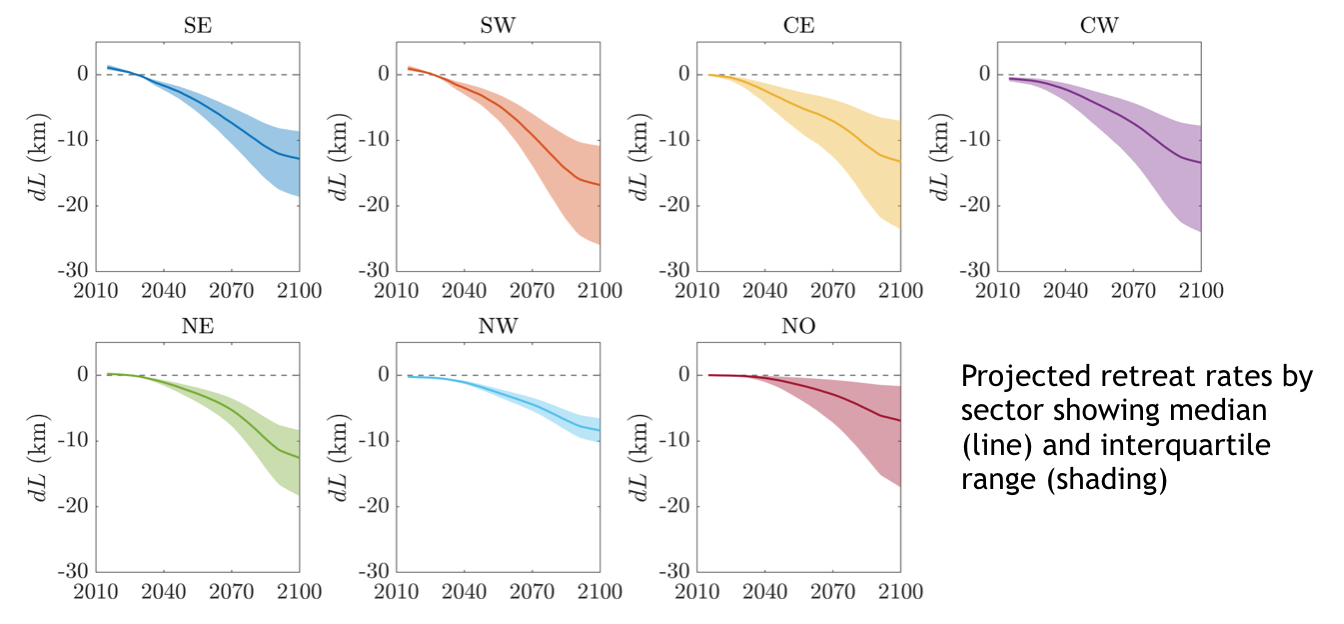
Figure 2: Example of the empirically-derived retreat scenarios for the 7 sectors of the Greenland ice sheet, obtained with MIROC5, RCP8.5.
As described in the webinar, retreat is imposed when the ice sheet geometry and ice front retreat scenario indicates that the land_ice_area_fraction_retreat mask is ice free for a given year. (Note the name was chosen so that it is closely related to the standard name land_ice_area_fraction -corresponding to variable name sftgif- in the ISMIP6 data request. For ease of communication, we use the longer standard name). Implementation for a specific ISM (also illustrated in Fig 3) requires the following steps:
- Identify ice prone to outlet glacier retreat, by interpolating initial ice mask conservatively to 1 km ISMIP6 diagnostic grid
to obtain a mask for ice fraction:
land_ice_area_fraction(x,y) = [0.0, …, 1.0]with 0.0 for ice free and 1.0 for ice covered - Calculate the distance to nearest ocean grid cell, or “distance_map”, based on model ice fraction and observed mask of ice with potential ocean contact ->
distance_map(x,y) - Calculate land ice fraction retreat based on distance map and retreat scenario:
land_ice_area_fraction_retreat(x,y,t) = [0.0, …, 1.0] with 0.0 for ice free and 1.0 for ice covered
- Interpolate
land_ice_area_fraction_retreatmask from diagnostic grid to model grid (conservatively) - Apply retreat in forward experiments (sub-grid implementation may be required for models with coarse resolutions to allow for partial retreat):
if land_ice_area_fraction_retreat(x,y,t) = 0.0, apply full retreat
if 0.0 < land_ice_area_fraction_retreat(x,y,t) < 1.0 apply partial retreat
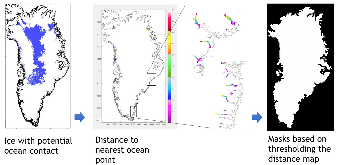 Figure 3: Illustration of the steps required for the implementation of the oceanic retreat.
ISMIP6 will generate the land_ice_area_fraction_retreat masks (steps 2-3) for each model. As retreat is provided as a series of ice fraction masks, ice sheet models with coarse resolution should use a sub-grid approach. A suggestion is to apply an land_ice_area_fraction_retreat that is relative to the reference thickness. Models may have a different strategy for this sub-grid implementation.
Note on the retreat dataset: the retreat rate dataset was calibrated using grounding line position of glaciers that do not have ice shelves. Although the retreat dataset is therefore not optimum for glaciers that have a floating tongue, it is suggested that retreat is imposed at the ice front. Modeling groups that have the capability of computing ice tongue basal melt may use the provided dataset of thermal forcing per basin.
To obtain the land_ice_area_fraction_retreat masks appropriate for your model, please submit your land_ice_area_fraction mask (step 1) to ISMIP6. This should be your ice mask from end 2014. We distinguish different cases to reduce interpolation artifacts:
- If your native grid is regular and on EPSG:3413, please provide your original modeled ice mask with x,y information
- If you have a high resolution irregular grid or a grid on a different projection than EPSG:3413, please get in touch so we can find the best solution for you. When ready, upload your file to the directory /ISMIP6/Projections/GrIS/Ocean_Forcing/Retreat_Implementation/MODELFILES/MODELNAME, where MODELNAME is the name of your model, and let us know via email that your file is uploaded.
ISMIP6 high resolution ocean melt rate allows ice sheet models to specify terminus retreat for each individual marine-terminating outlet glacier, thus allowing glaciers to retreat at different rates. This is accomplished by specifying a glacier terminus melt rate, calculated as a function of subglacial discharge (approximated as surface runoff from each glacier catchment) and ocean thermal forcing (Fig. 4). In addition to the melt rate, a calving rate must be specified to obtain the total frontal ablation rate at each terminus. As the dataset were created for an ice sheet geometry corresponding to present day observations from GIMP and BedMachine3, ISM that have differ substantially from this initial geometry should not use this dataset. (ie: if you are using Method 2 for the atmospheric forcing/SMB remapping, then the dataset is not applicable for your model, as the observed drainage basins used to generate the runoff field may not work with your model. You could create a dataset that is appropriate for your model from the remapped runoff and a water routing consistent with your geometry).
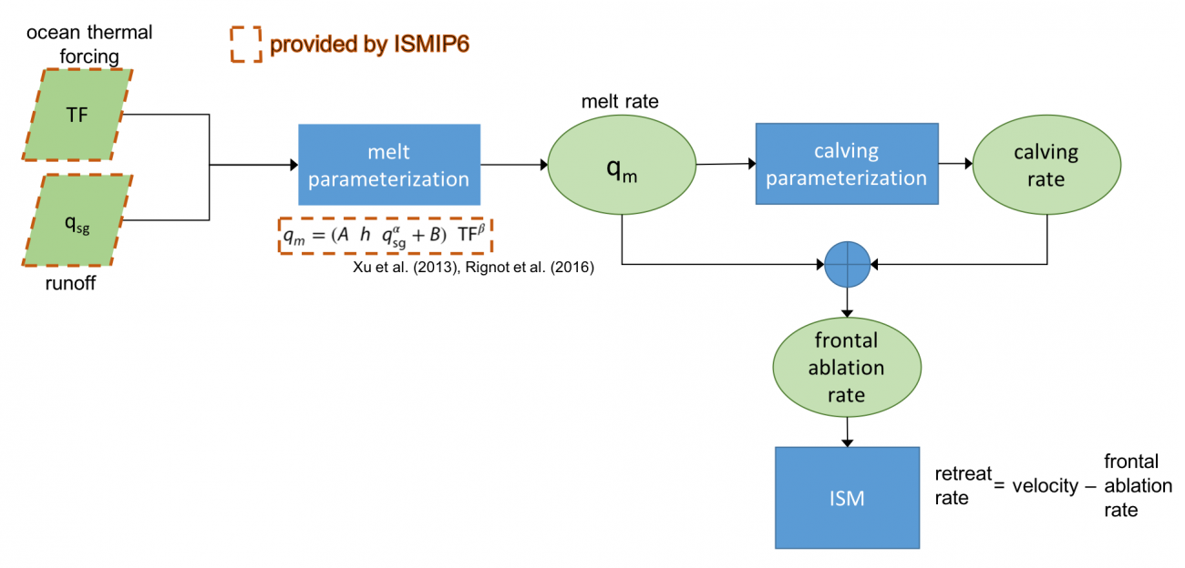
Figure 4: High-resolution melt-rate approach flow chart. Ocean thermal forcing and runoff fields are provided to the ice sheet modelers by the ISMIP6 ocean forcing working group. All parameters in the recommended melt-rate parameterization (Xu et al., 2013; Rignot et al., 2016) are provided, as well. Each ice sheet model must implement the approach and specify their own calving parameterization to calculate a frontal ablation rate for each outlet glacier.
ISMIP6 Open approach is used sample a larger variety of oceanic forcing parameterizations, as it remains an active field of research. Models are free to continue applying the ocean forcing parameterization they used during the model initialization or their preferred method, but should still rely on the ocean forcing datasets provided by ISMIP6 to simulate future ocean conditions.
Requirements for the projections
- Participants can and are encouraged to contribute with different models and/or initialisation methods
- Models have to be able to prescribe a given SMB anomaly
- Models have to be able to prescribe a given ice front retreat or the high resolution approach for the standard experiments. For the open experiments, models can choose the ocean parameterization of their choice but should use the ocean forcing provided.
- Adjustment of SMB due to geometric changes in forward experiments is encouraged using the provided dSMB/dz.
- Bedrock adjustment in forward experiment is allowed.
- The choice of model input data is unconstrained to allow participants the use of their preferred model setup without modification. Modelers without preferred data set choice can have a look at the Ghub ISMIP6 Browse Data page for possible options.
- To allow for analysis, any modeling choice needs to be well documented. A README file needs to be submitted along the outputs as an integral part of the contribution to the ISMIP6. It may be obtained here or requested by email to ismip6@gmail.com.
Appendix 1 – Output grid definition and interpolation
All 2D data is requested on a regular grid with the following description. Polar stereo-graphic projection with standard parallel at 70° N and a central meridian of 45° W (315° E) on datum WGS84 (EPSG3413 projection). The lower left cell center is at (-720000m,-3450000m) with nx=1681 and ny=2881 cells in x and y-direction at full km positions (xmin = -720 km, xmax = +960 km, ymin = -3450 km, ymax = -570 km). The output should be submitted on a resolution adapted to the resolution of the model and can be 20 km, 10 km, 5 km, 2 km or 1 km. The data will be conservatively interpolated to 1 km resolution for archiving and 5 km resolution for diagnostic processing by ISMIP6.
If interpolation is required in order to transform the SMB forcing to your native grid, and transform your model variables to the ISMIP6 output grid (20 km, 10 km, 5 km, 2 km, 1 km), it is required that conservative interpolation is used. The motivation for using a common method for all models is to minimize model to model differences due to the choice of interpolation method.
Note: The previously requested regular grid was in polar stereo-graphic projection with standard parallel at 71° N and a central meridian of 39° W (321° E) on datum WGS84. The lower left corner is at (-800000 m, -3400000 m) and the upper right at (700000 m, -600000 m). This is the same grid (Bamber et al., 2001) used to provide the SMB anomaly forcing previously. This grid was changed to the EPSG3413 projection described above.
A1.1 Regridding Tools and Tips
- An overview of the regridding process can be found on the two Regridding pages below.
- Regridding with CDO contains tools and tips that have been used by ISMIP6 members
- Regridding BISICLES output with ESMF and NCO contains other tools and tips
- ISMIP6 is designing tools to help with the regridding.
- If you need help with conservative interpolation, please email ismip6@gmail.com.
Appendix 2 – Naming conventions, upload and model output data.
Please provide:
- one variable per file for all 2D fields and scalar variables
- a completed readme file
A2.1 File name convention
File name convention for 2D fields and scalar variables:
<variable>_<IS>_<GROUP>_<MODEL>_<EXP>.nc
File name convention for readme file:
README_<IS>_<GROUP>_<MODEL>.doc
where
<variable> = netcdf variable name (e.g. lithk)
<IS> = ice sheet (AIS or GIS)
<GROUP> = group acronym (all upper case or numbers, no special characters)
<MODEL> = model acronym (all upper case or numbers, no special characters)
<EXP> = experiment name
For example, a file containing the variable “orog” for the Greenland ice sheet, submitted by group “JPL” with model “ISSM” for experiment “ctrl” would be called:
orog_GIS_JPL_ISSM_ctrl.nc
If JPL repeats the experiments with a different version of the model (for example, by changing the sliding law), it could be named ISSM2, and so forth.
When uploading your files to the server, please follow the standard directory structure.
Example:
- group1
- model1
- exp05_05
- expC01_05
- model1
- group2
- model2
- exp05_01
- expC01_01
- model2
Group, model and experiment names have to be identical in the directory names and file names, except for the resolution suffix (rr=[01, 05, ..] the resolution the submitted data in km).
Example for results at 1 km resolution:
AWI/ISSM1/ctrl_01/acabf_GIS_AWI_ISSM1_ctrl.nc
xxx yyyyy zzzz rr xxx yyyyy zzzz
The experiment names (exp_id) can be found at https://docs.google.com/spreadsheets/d/1YEiPV3Uc0K8EqD57mz-ZqBIF4XnVb5UbyRDRmox0KeE/edit#gid=1531275537
A few examples:
| exp_id | RCP | GCM | Ocean |
| exp 05 | 8.5 | MIROC5 | Medium |
| exp 06 | 8.5 | NorESM | Medium |
| exp a01 | 8.5 | IPSL-CM5-MR | Medium |
| exp b01 | ssp585 | CNRM-CM6 | Medium |
| exp c01 | 8.5 | MIROC5 AO | Medium |
| exp c01 | 8.5 | NorESM | High |
A2.2 Retrieving dataset and Uploading your model output
Accessing ISMIP6 datasets and Submitting model experiments
ISMIP6 datasets are distributed via the Ghub Globus web application. Public datasets can be found in Ghub’s Browse Data page. ISMIP6-specific initMIP Antarctic (and initMIP Greenland and projection data) can be accessed through the Ghub endpoints via Globus UI. To access and download data, one must create a Ghub account and register with Globus. Instructions to create accounts can be referenced in the General ISMIP6 Globus Instructions (v. 2023) instruction document at the end of this wiki.
All your model experiments can be uploaded via Globus/Ghub. See more details on Ghub’s Accessing Data wiki. Email ismip6 -at -gmail.com with any questions concerning the above.
The size of the model files on higher resolution grid can be largely reduced by file compression which will save space on the storage server. An example command is given below and the results before and after. In the examples that follow we can get a factor of 10 compression and for the masks even more given that contiguous masks are highly compressible because they are repeated data. NetCDF files have been designed with compression in mind. A NetCDF file can be compressed and nothing has to be changed in the way that it is read into Matlab or Python (or any other language that uses standard NetCDF read/write libraries).
The nccopy command copies an input netCDF file to an output netCDF file after compressing the file significantly. The ‘-d’ option stands for the deflation level, from 1 (faster but lower compression) to 9 (slower but more compression) and the ‘-s’ option is the shuffling option to improve compression even more. We recommend using ‘d1’ option since this option seems to accomplish the desired compression.
Example of netcdf compression command:
nccopy -d1 -s sftgif_GIS_JPL_ISSMPALEO_historical.nc sftgif_GIS_JPL_ISSMPALEO_historical_c.nc
Example of compression variant, seems to work better for masks:
nccopy -d1 sftgif_GIS_JPL_ISSMPALEO_historical.nc sftgif_GIS_JPL_ISSMPALEO_historical_c.nc
A2.3 Model output variables and README file
The README file is an important contribution to the ISMIP6 submission. It may be obtained here or requested by email to ismip6@gmail.com
A2.3.1 General guidelines The variables requested in the table below serve to evaluate and compare the different models and initialization techniques. Some of the variables may not be applicable for your model, in which case they are to be omitted (with explanation in the README file). Also, specify missing values in your netcdf file where needed, and fields should be undefined outside of the ice mask.
All “missing data” must be assigned the single precision floating point value of 1.e20
We distinguish between state variables “ST” (e.g. ice thickness, temperatures and velocities) and flux variables “FL” (e.g. SMB). State variables should be given as snapshot information at the end of one year for both scalars and 2D variables (for initMIP, 2D variables were only requested over five year periods), while flux variables are to be averaged over the respective periods. Please specify in your README file how your reported flux data has been averaged over time. Ideally, the standard would be go average over all native time steps.
Flux variables are defined positive when the process adds mass to the ice sheet and negative otherwise.
If you redo the initMIP experiments (because you have a new initial state for the projections), please save the files at a yearly interval instead of the 5 years interval requested as part of the original initMIP. Also upload your iniMIP results in the projections directory.
A2.3.2 How to record time in historical and projection files
In compliance with CMIP6, time should be defined in “days since “, where must be specified by the user, typically in the form year-month-day (e.g., “days since 1800-1-1”). For simulations meant to represent a particular historical period, set the ‘base time’ to the time at the beginning of the simulation. A historical run initialized with forcing for year 2007 would, for example, have units of “days since 2007-1-1”. For the future scenario runs, retain the same as used in the historical run from which it was initiated. Note the CF definition for years (section 4.4): a common_year is 365 days, a leap_year is 366 days, a Julian_year is 365.25 days, a Gregorian_year is 365.2425 days, a 360_day has all years with 360 days divided into 30 day months (please see the CF link above for other examples on calendar setting in section 4.4).
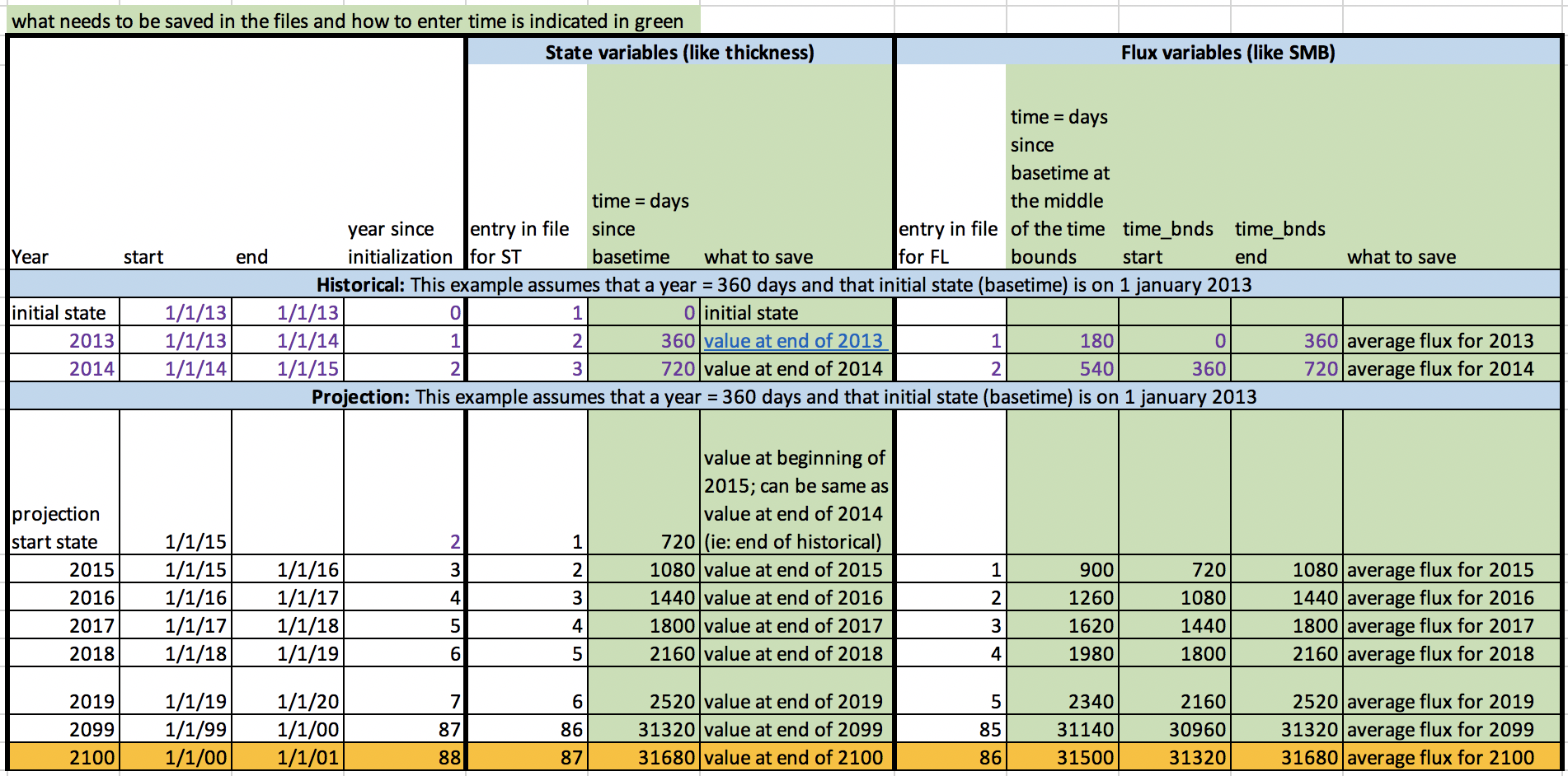
To illustrate a time recording for the historical file and projections for a typical state variable (ST, eg thickness) and flux variable (FL, eg SMB), we assume that our <basetime> is January 1st 2013, and that we use a calendar = 360_days. Other calendars can be used, but you need to indicate the calendar used in the netcdf, and of course if you use a different calendar, the time entries will be different. What needs to be recorded is shown in green in the Table below. For state variables, is the day corresponding to the entry that you are saving since the your <basetime>. For flux variables, since these are averaged over a year, is the day since <basetime> corresponding to the middle of the year, while <time_bnds> records the day since <basetime> at the start and end of a year. Note that in CMIP a full year is typically from first of January to the first of January of the following year. We also provide below example of what the netcdf would look like for our example..
For state variables, like thickness for the historical:
 dimensions:
    time = UNLIMITED ; // (3 currently)
 variables:
    double time(time) ;
        time:units = "days since 1-1-2013" ; // This date correspond to the example basetime
        time:calendar = "360_day" ; // Other calendars can be used... change here to relevant calendar
        time:axis = "T" ;
        time:long_name = "time" ;
        time:standard_name = "time" ;
 data:
  time = 0, 360, 720; // If you use a different calendar these values will change

and thickness for the projection (note that the full time entries are not shown, only beginning and end) would be:
 dimensions:
    time = UNLIMITED ;
 variables:
    double time(time) ;
        time:units = "days since 1-1-2013" ; // This date correspond to the example basetime
        time:calendar = "360_day" ; // Other calendars can be used... change here to relevant calendar
        time:axis = "T" ;
        time:long_name = "time" ;
        time:standard_name = "time" ;
 data:
  time = 720, 1080, 1440, …, 31320, 31680; // If you use a different calendar these values will change

The flux variable, like SMB, would be recorded as the average over a full year, so for the historical:
 dimensions:
    time = UNLIMITED ; // (2 currently)
    bnds = 2 ;
 variables:
    double time(time) ;
        time:bounds = "time_bnds" ;
        time:units = "days since 1-1-2013 " ; // This date correspond to the example basetime
        time:calendar = "360_day" ; // Other calendars can be used... change here to relevant calendar
        time:axis = "T" ;
        time:long_name = "time" ;
        time:standard_name = "time" ;
    double time_bnds(time, bnds) ;
 data:
  time = 180, 540 ; // If you use a different calendar these values will change.
                              //This is the middle of the time_bnds
  time_bnds =
   0, 360, //If you use a different calendar these values will change.
               //These are the day since basetime at the beginning and end of the year
   360, 720 ;

and the projection (note that the full time entries are not shown, only beginning and end):
 dimensions:
    time = UNLIMITED ; //
    bnds = 2 ;
 variables:
    double time(time) ;
        time:bounds = "time_bnds" ;
        time:units = "days since 1-1-2013 " ; // This date correspond to the example basetime
        time:calendar = "360_day" ;  // Other calendars can be used... change here to relevant calendar
        time:axis = "T" ;
        time:long_name = "time" ;
        time:standard_name = "time" ;
    double time_bnds(time, bnds) ;
 variables:
    double time(time) ;
        time:bounds = "time_bnds" ;
 data:
  time = 900, 1260, 1620, ..., 31140, 31500; // If you use a different calendar these values will change.
                                                      //This is the middle of the time_bnds
  time_bnds =
 720, 1080, //If you use a different calendar these values will change.
                  //These are the day since basetime at the beginning and end of the year
 1080, 1440,
 1440, 1800,
 ....
 30960, 31320,
 31320, 31680;
A2.3.3 Table A1: Variable request for ISMIP6
If your quantity does not change with time, then simply save one time entry. An example is geothermal heat flux, which varies in some models but not others.
| Variable | Dim | Type | Variable Name | Standard Name | Units | Comment |
| 2D variables requested yearly as snapshots (end of the year) for type ST and as yearly average for type FL. | ||||||
| Ice thickness | x,y,t | ST | lithk | land_ice_thickness | m | The thickness of the ice sheet |
| Surface elevation | x,y,t | ST | orog | surface_altitude | m | The altitude or surface elevation of the ice sheet |
| Bedrock elevation | x,y,t | ST | topg | bedrock_altitude | m | The bedrock topography (may change during the projections) |
| Geothermal heat flux | x,y,t | FL | hfgeoubed | upward_geothermal_heat_flux_in_land_ice alias upward_geothermal_heat_flux_at_ground_level | W m-2 | Geothermal Heat flux at the ice interface (only needed beneath the grounded ice). If this quantity does not change with time simply enter one timestep |
| Surface mass balance flux | x,y,t | FL | acabf | land_ice_surface_specific_mass_balance_flux | kg m-2 s-1 | Surface Mass Balance flux (for areas covered by ice only) |
| Basal mass balance flux beneath grounded ice | x,y,t | FL | libmassbfgr alias “libmassbf” | land_ice_basal_specific_mass_balance_flux | kg m-2 s-1 | Basal mass balance flux (only beneath grounded ice) |
| Basal mass balance flux beneath floating ice | x,y,t | FL | libmassbffl alias “libmassbf” | land_ice_basal_specific_mass_balance_flux | kg m-2 s-1 | Basal mass balance flux (only beneath floating ice) |
| Ice thickness imbalance | x,y,t | FL | dlithkdt | tendency_of_land_ice_thickness | m s-1 | dHdt |
| Surface velocity in x | x,y,t | ST | xvelsurf alias “uvelsurf” | land_ice_surface_x_velocity | m s-1 | u-velocity at land ice surface |
| Surface velocity in y | x,y,t | ST | yvelsurf alias “vvelsurf” | land_ice_surface_y_velocity | m s-1 | v-velocity at land ice surface |
| Surface velocity in z | x,y,t | ST | zvelsurf alias “wvelsurf” | land_ice_surface_upward_velocity | m s-1 | w-velocity at land ice surface |
| Basal velocity in x | x,y,t | ST | xvelbase alias “uvelbase” | land_ice_basal_x_velocity | m s-1 | u-velocity at land ice base |
| Basal velocity in y | x,y,t | ST | yvelbase alias “vvelbase” | land_ice_basal_y_velocity | m s-1 | v-velocity at land ice base |
| Basal velocity in z | x,y,t | ST | zvelbase alias “wvelbase” | land_ice_basal_upward_velocity | m s-1 | w-velocity at land ice base |
| Mean velocity in x | x,y,t | ST | xvelmean alias “uvelmean” | land_ice_vertical_mean_x_velocity | m s-1 | The vertical mean land ice velocity is the average from the bedrock to the surface of the ice |
| Mean velocity in y | x,y,t | ST | yvelmean alias “vvelmean” | land_ice_vertical_mean_y_velocity | m s-1 | The vertical mean land ice velocity is the average from the bedrock to the surface of the ice |
| Surface temperature | x,y,t | ST | litemptop alias “litempsnic” | temperature_at_top_of_ice_sheet_model alias “temperature_at_ground_level_in_snow_or_firn” | K | Ice temperature at surface |
| Basal temperature beneath grounded ice sheet | x,y,t | ST | litempbotgr alias “litempbot” | temperature_at_base_of_ice_sheet_model alias “land_ice_basal_temperature” | K | Ice temperature at base of grounded ice sheet |
| Basal temperature beneath floating ice shelf | x,y,t | ST | litempbotfl alias “litempbot” | temperature_at_base_of_ice_sheet_model alias “land_ice_basal_temperature” | K | Ice temperature at base of floating ice shelf |
| Basal drag | x,y,t | ST | strbasemag | land_ice_basal_drag alias “magnitude_of_land_ice_basal_drag” | Pa | Basal drag |
| Calving flux | x,y,t | FL | licalvf | land_ice_specific_mass_flux_due_to_calving | kg m-2 s-1 | Loss of ice mass resulting from iceberg calving. Only for grid cells in contact with ocean |
| Ice front calving and melt flux | x,y,t | FL | lifmassbf | land_ice_specific_mass_flux_due_to_calving_and_ice_front_melting | kg m-2 s-1 | Loss of ice mass resulting from calving and ice front melting. Only for grid cells in contact with ocean |
| Land ice area fraction | x,y,t | ST | sftgif | land_ice_area_fraction | 1 | Fraction of grid cell covered by land ice (ice sheet, ice shelf, ice cap, glacier) |
| Grounded ice sheet area fraction | x,y,t | ST | sftgrf | grounded_ice_sheet_area_fraction | 1 | Fraction of grid cell covered by grounded ice sheet, where grounded indicates that the quantity correspond to the ice sheet that flows over bedrock |
| Floating ice sheet area fraction | x,y,t | ST | sftflf | floating_ice_shelf_area_fraction alias “floating_ice_sheet_area_fraction” | 1 | Fraction of grid cell covered by ice sheet flowing over seawater |
| Scalar outputs requested every full year: snapshots for type ST and 1 year averages for type FL. | ||||||
| Total ice mass | t | ST | lim | land_ice_mass | kg | spatial integration, volume times density |
| Mass above floatation | t | ST | limnsw | land_ice_mass_not_displacing_sea_water | kg | spatial integration, volume times density |
| Grounded ice area | t | ST | iareagr alias “iareag” | grounded_ice_sheet_area | m2 | spatial integration |
| Floating ice area | t | ST | iareafl alias “iareaf” | floating_ice_shelf_area | m2 | spatial integration |
| Total SMB flux | t | FL | tendacabf | tendency_of_land_ice_mass_due_to_surface_mass_balance | kg s-1 | spatial integration |
| Total BMB flux | t | FL | tendlibmassbf | tendency_of_land_ice_mass_due_to_basal_mass_balance | kg s-1 | spatial integration |
| Total BMB flux beneath floating ice | t | FL | tendlibmassbffl | tendency_of_land_ice_mass_due_to_basal_mass_balance | kg s-1 | spatial integration (computed beneath floating ice only) |
| Total calving flux | t | FL | tendlicalvf | tendency_of_land_ice_mass_due_to_calving | kg s-1 | spatial integration |
| Total calving and ice front melting flux | t | FL | tendlifmassbf | tendency_of_land_ice_mass_due_to_calving_and_ice_front_melting | kg s-1 | spatial integration |
Appendix 3 – Participating Models and Characteristics
Greenland Standalone Ice Sheet Modeling
| Contributors | Model | Group ID | Group |
| Martin Rückamp, Angelika Humbert | ISSM | AWI | Alfred Wegener Institute for Polar and Marine Research, DE /University of Bremen, DE |
| Victoria Lee, Tony Payne, Stephen Cornford, Daniel Martin | BISICLES | BGC | University of Bristol, Bristol, UK, Department of Geography, Swansea University, UK, Computational Research Division, Lawrence Berkeley National Laboratory, California, USA |
| Isabel Nias, Sophie Nowicki, Denis Felikson | ISSM | GSFC | NASA Goddard Space Flight Center, Greenbelt, USA |
| Ralf Greve, Reinhard Calov, Chris Chambers | SICOPOLIS | ILTS_PIK | Institute of Low Temperature Science, Hokkaido University, Sapporo, JP, Potsdam Institute for Climate Impact Research, Potsdam, DE |
| Heiko Goelzer, Roderik van de Wal, Michiel van den Broeke | IMAUICE | IMAU | Utrecht University, Institute for Marine and Atmospheric Research (IMAU), Utrecht, NL |
| Helene Seroussi, Nicole Schlegel | ISSM | JPL | NASA Jet Propulsion Laboratory, Pasadena, USA |
| Joshua K. Cuzzone, Nicole Schlegel | ISSMPALEO | JPL | NASA Jet Propulsion Laboratory, Pasadena, USA |
| Aurélien Quiquet, Christophe Dumas | GRISLI | LSCE | LSCE/IPSL, Laboratoire des Sciences du Climat et de l’Environnement, CEA-CNRS-UVSQ, Gif-sur-Yvette, FR |
| Lev Tarasov | GSM | MUN | Dept of Physics and Physical Oceanography, Memorial University of Newfoundland, USA |
| William Lipscomb, Gunter Leguy | CISM | NCAR | National Center for Atmospheric Research, Boulder, CO USE |
References
Barthel, A., Agosta, C., Little, C.M., Hattermann, T., Jourdain, N.C., Goelzer, H., Nowicki, S., Seroussi, H., Straneo, F. and Bracegirdle, T.J., (2020). CMIP5 model selection for ISMIP6 ice sheet model forcing: Greenland and Antarctica, The Cryosphere, 14, 855–879, https://doi.org/10.5194/tc-14-855-2020
Franco, B., Fettweis, X., Lang, C., and Erpicum, M.: Impact of spatial resolution on the modelling of the Greenland ice sheet surface mass balance between 1990–2010, using the regional climate model MAR, The Cryosphere, 6, 695-711, https://doi.org/10.5194/tc-6-695-2012, 2012.
Goelzer, H., Nowicki, S., Edwards, T., Beckley, M., Abe-Ouchi, A., Aschwanden, A., Calov, R., Gagliardini, O., Gillet-Chaulet, F., Golledge, N. R., Gregory, J., Greve, R., Humbert, A., Huybrechts, P., Kennedy, J. H., Larour, E., Lipscomb, W. H., Le clec’h, S., Lee, V., Morlighem, M., Pattyn, F., Payne, A. J., Rodehacke, C., Rückamp, M., Saito, F., Schlegel, N., Seroussi, H., Shepherd, A., Sun, S., van de Wal, R., and Ziemen, F. A.: Design and results of the ice sheet model initialisation experiments initMIP-Greenland: an ISMIP6 intercomparison, The Cryosphere, 12, 1433-1460, https://doi.org/10.5194/tc-12-1433-2018, 2018.
Goelzer, H., Noel, B. P. Y., Edwards, T. L., Fettweis, X., Gregory, J. M., Lipscomb, W. H., van de Wal, R. S. W., and van den Broeke, M. R. (2020). Remapping of Greenland ice sheet surface mass balance anomalies for large ensemble sea-level change projections, The Cryosphere, 14, 1747–1762, https://doi.org/10.5194/tc-14-1747-2020.
Le clec’h, S., Charbit, S., Quiquet, A., Fettweis, X., Dumas, C., Kageyama, M., Wyard, C., and Ritz, C.: Assessment of the Greenland ice sheet–atmosphere feedbacks for the next century with a regional atmospheric model coupled to an ice sheet model, The Cryosphere, 13, 373-395, https://doi.org/10.5194/tc-13-373-2019, 2019.
Nowicki, S., Goelzer, H., Seroussi, H., Payne, A. J., Lipscomb, W. H., Abe-Ouchi, A., Agosta, C., Alexander, P., Asay-Davis, X. S., Barthel, A., Bracegirdle, T. J., Cullather, R., Felikson, D., Fettweis, X., Gregory, J. M., Hattermann, T., Jourdain, N. C., Kuipers Munneke, P., Larour, E., Little, C. M., Morlighem, M., Nias, I., Shepherd, A., Simon, E., Slater, D., Smith, R. S., Straneo, F., Trusel, L. D., van den Broeke, M. R., and van de Wal, R. (2020). Experimental protocol for sea level projections from ISMIP6 stand-alone ice sheet models, The Cryosphere, 14, 2331–2368, https://doi.org/10.5194/tc-14-2331-2020
Rignot, E., Xu, Y., Menemenlis, D., Mouginot, J., Scheuchl, B., Li, X., et al.: Modeling of ocean-induced ice melt rates of five west Greenland glaciers over the past two decades. Geophysical Research Letters, 43(12). http://doi.org/10.1002/2016GL068784, 2016.
Shannon, S.R., Payne A.J., Bartholomew I.D., Van Den Broeke M.R., Edwards T.L., Fettweis X., Gagliardini O., Gillet-Chaulet F., Goelzer H., Hoffman M.J., Huybrechts P.: Enhanced basal lubrication and the contribution of the Greenland ice sheet to future sea-level rise, Proceedings of the National Academy of Sciences, 110(35):14156-61. https://doi.org/10.1073/pnas.1212647110, 2013.
Slater, D. A., Straneo, F., Felikson, D., Little, C. M., Goelzer, H., Fettweis, X., and Holte, J. (2019). Estimating Greenland tidewater glacier retreat driven by submarine melting, The Cryosphere, 13, 2489–2509, https://doi.org/10.5194/tc-13-2489-2019.
Slater, D. A., Felikson, D., Straneo, F., Goelzer, H., Little, C. M., Morlighem, M., Fettweis, X., and Nowicki, S. (2020). 21st century ocean forcing of the Greenland Ice Sheet for modeling of sea level contribution, The Cryosphere, 14, 985–1008, https://doi.org/10.5194/tc-14-985-2020.
Xu, Y., Rignot, E., Fenty, I., Menemenlis, D., & Flexas, M. M.: Subaqueous melting of Store Glacier, west Greenland from three-dimensional, high-resolution numerical modeling and ocean observations. Geophysical Research Letters, 40(17). http://doi.org/10.1002/grl.50825, 2013.
Acknowledgements
The experimental protocol and datasets for the ISMIP6-Projections-Greenland standalone ice sheet simulations would not have been possible without the effort of many scientists that have given their time and expertise, and have run models to convert the CMIP5 models output into datasets that standalone ice sheet models can use. ISMIP6 would like to thank the ocean focus group under the leadership of Fiamma Straneo, the atmospheric focus group under the leadership of Bill Lipscomb and Robin Smith, and the CMIP5 model evaluation focus group under the leadership of Alice Barthel. Donald Slater, Denis Felixson, Mathieu Morlinghem and Heiko Goelzer have been instrumental in the development of the ice front retreat and melt parameterization and associated dataset. Xavier Fettweis, Patrick Alexander and Heiko Goelzer prepared the atmospheric dataset. Alice Barthel, Chris Little, Cecile Agosta, and Jamie Holte provided a rigorous analysis of the CMIP5 models against historical data, which allowed the CMIP5 model evaluation group and the ISMIP6 steering committee to select the CMIP5 models used in this effort. Finally, we thank the ISMIP6 ice sheet modelers for their feedback on the design of the protocol and their willingness to participate in ISMIP6.
General ISMIP6 Globus Instructions (v. 2023): Globus_Instructions_ismip6_general_June2023.docx (2 MB, uploaded by Katelyn Eaman 1 year 2 months ago).